Current World Environment

Introduction

Air pollution is the biggest climate change issue nowadays, and predicting air quality helps to warn and control pollution. The nitrogen oxide (NOX) and air quality index (AQI) levels were estimated over Beijing and Italy using random forest regression (RFR)¹. Maharashtra's COVID-19 shutdown lowered PM_2.5, PM₁₀, NO₂, and CO levels. Ammonia released from agriculture fields as livestock waste and other fertilizers, when it is released into the atmosphere, can react with acid compounds to form ammonium

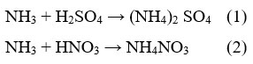
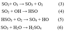
Haze, consisting of ammonium compounds, obscures natural landscapes and reduces their aesthetic value. The transformation of ammonia into these substances can lead to acid rain, which can harm plants, aquatic ecosystems, and structures. The burning of fossil fuels and industrial processes are primary sources of sulfur dioxide emissions into the atmosphere, resulting from the reaction of ozone and hydroxyl radicals (OH). While HSO₃ is being oxidized, sulfur trioxide is released. This reacts with water (H₂O) to make the acidic compound H₂SO₄.

Surface ozone (O₃) is generated by two main processes: stratospheric intrusion and in-situ photochemical decay of carbon-linked molecules (such as CO, CH₄, and Volatile organic compounds) in the existence of NOx³⁰. Mechanism of Ozone (O₃) production from following reaction

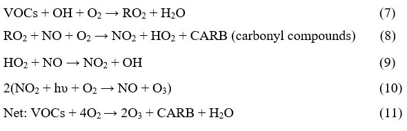
The primary sources of O₃ precursor gases include biomass combustion, fossil fuel combustion, and several other human activities. The photochemical reaction of precursor gases i.e., nitrogen oxides (NOx) forms Ozone (O₃) in the troposphere³¹. But the chemical process that leads to the formation of O₃ is very non-linear. Global divergent forcing is rising by +0.35 W/m² owing to ozone in the troposphere. However, due to regional weather patterns, the AQI remained high.² The air quality has improved in 70% of locations due to the COVID-19 lockdowns.

The areas of India that have seen the most improvement is Western, Northern, and Eastern India.³ Better public transportation, cleaner fuels, and waste management are all long-term solutions that Delhi needs to combat its air pollution problem, which persists throughout the year. To solve the problem, a centralized agency, monitoring, and urban planning are essential.⁴ The burning of coal and wood is the main cause of the winter haze that severely affects the air quality in Amravati Town. The study utilizes the Random Forest Regression (RFR) model for accurate estimation. ⁵ The most successful prediction model for detecting and predicting air quality in this study is decision tree regression. Governments and researchers must work together to create regulations for managing air quality.⁶ Air pollution levels must be controlled due to rapid urbanization. The most effective method for identifying air quality and forecasting future AQI levels, according to the results, is decision tree regression.⁷ Furthermore, the majority of nations use fixed monitoring stations that are centralized for their urban air quality monitoring systems. In order to forecast air pollution, scientists have worked to create and refine models that track airborne contaminants. The objective of this study is to predict the precision and outcome of the model by making use of all the labeled data. This article looked at a variety of regression models to find the best model for air quality forecast systems. It describes how collecting data on pollution concentrations from CPCB for the Python language makes it possible to predict the state of the air and develop model for air quality.

Machine learning and its modules

The best model is artificial intelligence, which is characterized by an element's ability to sense, reason, prefer, and learn from its mistakes. ML, a subfield of AI, enables components to learn without explicit programming with predetermined rules.⁸ A machine learning model is a technique that examines input data to determine how it relates to a desired value, which is related to the training data set.

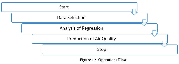Figure 1: Operations Flow Click here to view Figure

We refer to it as testing when we apply the model to previously unseen new inputs to evaluate the learned relationship.⁹  Models must possess both low bias and low variance, as this is crucial. By adjusting the hyperparameters, researchers can optimize the ML model algorithm and reduce loss when applied to a specific dataset.

Machine learning methods

It is a specific subdivision of artificial intelligence whose purpose is to free the computer from explicit rule programming so that it can learn on its own. A machine learning system can model and forecast the world by finding and understanding underlying patterns in observed data. Supervised algorithms, in contrast to simpler but non-trained unsupervised learning techniques, require human input, output, and feedback during training and reinforcement learning, unsupervised learning, and supervised learning are the three types of machine learning that we use in our methodologies¹⁰. The following process represents a step of data analysis that involves modeling to predict air quality.

Linear regression

Every introduction to machine learning should begin with a discussion of linear regression models since they are straightforward but very effective. One important aspect of this approach is that it only takes one numerical value—the ratio of the change in the predictor to the modification in the response—to describe each predictor variable's contribution to the outcome statistic. Because it is assumed that all impacts are linear, this degree of simplicity is achievable.¹¹ When two independent or response variables are paired with one dependent or predictor variable, the analysis is referred to as simple regression. In certain situations, straight lines of the following shape fit by a linear regression analysis:

or in another word

The constant term (C), commonly known as the "intercept," represents the value of the response variable when the predictor is equal to zero. The coefficient (B) is a mathematical expression that quantifies the relationship between the change in the reaction and the change in the forecasting factor. Sometimes, people refer to it as a weight or a slope coefficient²⁹.

Decision Tree regression

The most powerful algorithm in machine learning, the decision tree, is also the most straightforward. It is a member of the supervised learning algorithm family. Regression and classification issues can also be resolved with the decision tree method. A decision tree (DT) is progressively created as a result of dividing the dataset into smaller subgroups. Consequently, decision nodes and leaf nodes can be found in the final resultant tree. The algorithm's output is represented by leaf nodes, while decision nodes indicate a condition.

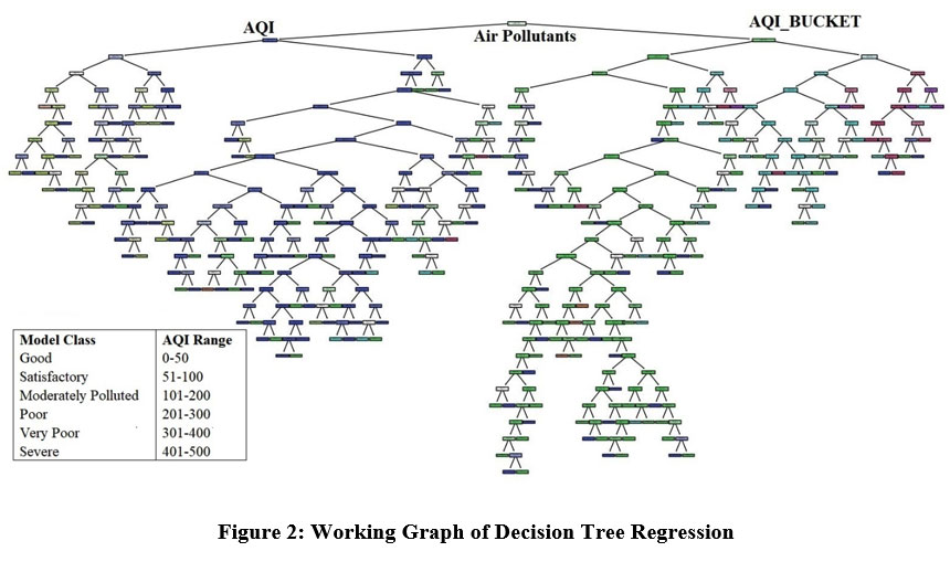Figure 2: Working Graph of Decision Tree Regression. Click here to view Figure

Moreover, decision trees are employed in two categories: (i) problems with categorical output and (ii) problems with continuous output. Regression using decision trees is applied to the continuous output problem. The algorithm selects the characteristics of an object and constructs a model using a tree structure. The trained model assists in predicting future data so that the necessary output can be produced. A functional example of decision tree regression is presented in Figure 2.

Random Forest regression

Ensemble learning techniques for classification, regression, and other tasks are called random forests (RFR). Growing classification and regression trees are used to produce the mean prediction of individual trees or the mode of classes after building several decision trees at various training times. The study determines the number of decision trees before training the model. A greater number is preferable in terms of trees, but it requires more computing power. Lower NF values are associated with greater variance reduction and higher bias increase.¹

Author can use the empirical formula to define NF = /M, where M represents the total number of features. Regression trees or classification trees can use RF to solve both classification and regression problems. Figure 3 also displays the regression model. The final output of the regression model is the following: The model takes into account the presence of regression trees, also known as learners, in the regression prediction process.

where T denotes the total count of regression trees and hi(x) represents the output of the i^th tree tested on sample x. As a result, the average of all the trees' predicted values represents the RF prediction.

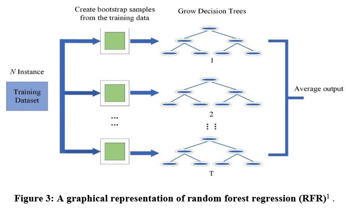Figure 3: A graphical representation of random forest regression (RFR) . Click here to view Figure

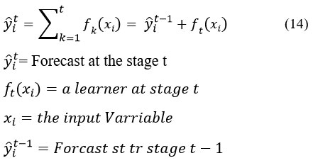
Extreme gradient boosting (XGBoost)

The process of combining several inefficient classifiers into a single powerful one is referred to as "boosting." The application of Gradient Boosting served as the basis for the development of the XGBoost methodology¹². When it comes to computational efficiency, scalability, and generalization performance, the XGBoost version of Gradient Boosting is superior to the original version. When working with XGBoost, proficient data management is of the utmost importance. Due to the fact that XGBoost only accepts numeric vectors as input, all categorical data will be transformed into the numerical values that correspond to them. Using a one-hot encoding is one method that can be utilized to accomplish this transformation. The present investigation is able to acquire the estimated model by employing the universal function, as demonstrated by the form that is presented below:           

Metrics for performance:

Equation (15, 16) illustrates the two statistical indicators that were used to examine the performance of supervised techniques models.

Root Mean Square Error (RMSE): The term RMSE refers to the square root of the mean squared error. It determines the standard deviation to represent the residual dispersion. It selects an object's attributes and uses a tree's structure to train a model.

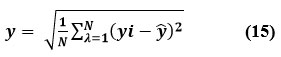
The R-squared value evaluates how effectively a linear regression model explains changes in the dependent variable. While it is scale-free, or unaffected by the magnitude of the data, it remains below one. In this case, y is the average value of y, and Y is the estimated amount of y by the equation¹³ .

Literature review

Methodology

The Central Pollution Control Board (CPCB) provided data for eight cities in Rajasthan, i.e., Jodhpur, Kota, Udaipur, Ajmer, Pali, Bhiwandi, and Alwar, for the years 2019–2023. This study measured the concentrations of air pollutants at these locations. The analysis aims to determine the pollution levels in the western part of India before, during, and after the COVID-19 event.

Data Source

The study used air quality data from Udaipur, Jaipur, Ajmer, Alwar, Bhiwandi, Jodhpur, Pali, and Kota cities to assess the air quality of Rajasthan during the pre-lockdown (before), lockdown (during), and post-lockdown (after) phases. This data, received directly from the Central Pollution Control Board web page (https://cpcb.nic.in/), contained measurements of particulate matter, sulfur dioxide, nitrogen dioxide (NO₂), carbon monoxide, and ozone (O₃).

Data Methodology

Data mining is a process that converts raw data into more easily understandable formats by filling in missing values or reducing data noise. To evaluate models, it is crucial to split datasets into training and testing sets. The testing set, which accounts for 80% of the data, is primarily used for assessment, while the remaining 20% is used for training. This approach helps to elucidate model characteristics and minimize data discrepancies..

Result and Discussion

Variation of AQI Concentration for City

(Pre-lockdown and Lockdown)

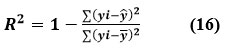
The present study used three months of data from the CPCB for the seven pollutants and AQI in the months of March , April and May during a five-year period that included 2019 (before), 2020 (during), and 2021–2023 (after).When comparing pre-lockdown versus lockdown implemented for three months in March, April, and May of 2019 and 2020, cities significantly lowered the AQI values, with maximum and minimum reductions observed in the state of Rajasthan (Fig. 4 and Table 1), particularly in the AQI concentration of Alwar and Jodhpur. The average concentrations of Alwar have dropped by around (-35.6%).The reduction in particle levels was largely due to unexpected local emissions as well as meteorological factors like rainfall and air mass movement²⁰. Other concentrations that have clearly varied between pre-lockdown and lockdown are Ajmer (-22.02%) and Bhiwandi (-21.79%) soon. Regretfully, there was no discernible trend, and the drops were quite tiny in Udaipur and Jodhpur (-9.12% and -8.1%) (Fig. 2). The tendency of the Jaipur AQI (+7.2%) total variation has strengthened during the course of the research period.

Table 1: Overall variation of percentage change

Figure 4: There were overall percentage changes in the AQI in March, April, and May of 2019 and 2020 during the pre-lockdown and lockdown periods. Click here to view Figure

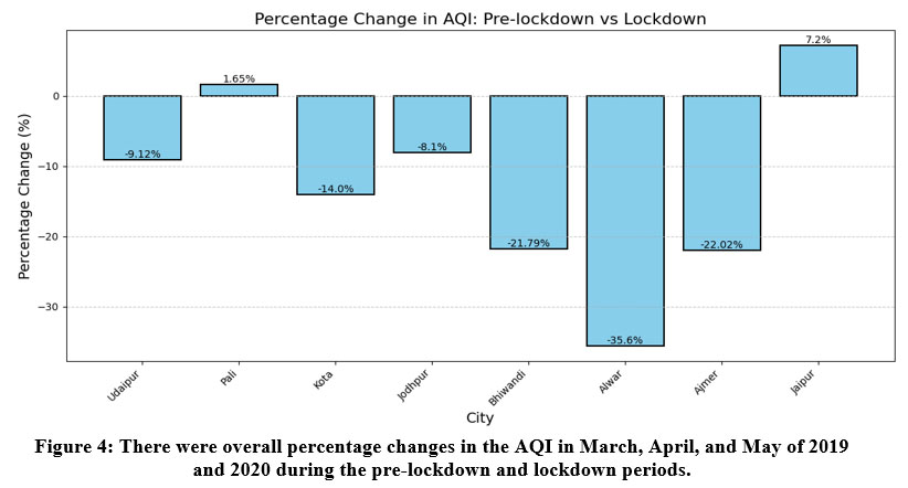
Figure 5 depicted the study period of 2020 as under lockdown, and the study periods of 2021, 2022, and 2023 as post-lockdown for three months in March, April, and May. During this time, the cities in the state of Rajasthan had significantly higher AQI values for both the maximum and minimum increments (Fig. 5 and Table 1), especially in the AQI concentrations of Jaipur and Alwar. There has been about an 86.77% increase in the average concentrations in Jaipur. Vehicle traffic, low tree density, and excess construction of buildings may increase pollution concentrations in Jaipur²¹.Kota (75.99%) and Pali (61.72%) are two other concentrations that have obviously changed between lockdown and post-lockdown, respectively. Unfortunately, there was no increasing trend, and the highest percentages were insignificant in Ajmer and Alwar (16.83% and 4.12%) (Fig. 5).

Figure 5: The AQI's overall percentage change in March, April, and May between Lockdown (2020) and post-lockdown (2021, 2022, and 2023). Click here to view Figure

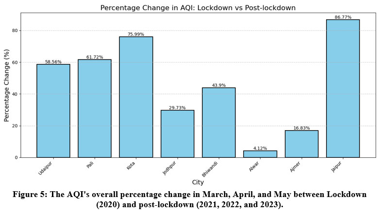
Deep Learning Study on Air Quality Index and Air Pollutants Using

Stack Model Heat Map (Seaborn).

The Air Quality Index (AQI) study used these three months of data from the CPCB. During the study period, the author collected these months, March, April, and May, over a five-year period that encompassed 2019, 2020, and 2021–2023. As shown in Figures 6, 7, and 8, the contaminants (PM₁₀, PM_2.5, NO₂, NH₃, SO₂, O₃, and CO) were measured before, during, and after the lockdown. The AQI classification was shown by a Seaborn Pair plot. The AQI class categorization, which uses Python, includes the following values: The range of values includes excellent (0 to 50), acceptable (51 to one 100), moderately polluted (101 to 200), poor (201 to 300), very poor (301 to 400), and severe (> 400).The study displays a correlation between the variable distribution and the AQI. It is clear from the study period that during lockdown, there is a positive correlation between the air pollutants excluded, ozone (O₃) and carbon monoxide (CO). PM_2.5 and PM₁₀ showed the highest degree of correlation. The results from the pair plot under satisfactory and moderately polluted conditions indicated an development in the air quality in the western part of India. Researchers from around the world ^22–26 have found that the quality of the air is better now than it was before the pre-lockdown in 2019, as shown in Figure 6. Figure 7 illustrates how air pollution levels can shift from moderately polluted to very poor when correlated with PM_2.5, PM₁₀, and AQI data. This alteration could have been triggered by dust activities and high temperature. The increase in class satisfaction in the event of a lockdown indicates that the AQI values are improving. The research highlights the advantages of using deep learning for short-term air pollution predictions. A remarkable growth is reflected in Post-lockdown with falling under Moderately Polluted to Very Poor conditions as shown in fig.8.

Figure 6: Air Pollution and Air quality Index (Stack Model Heat Map - Seaborn) pre-lockdown in 2019. Click here to view Figure

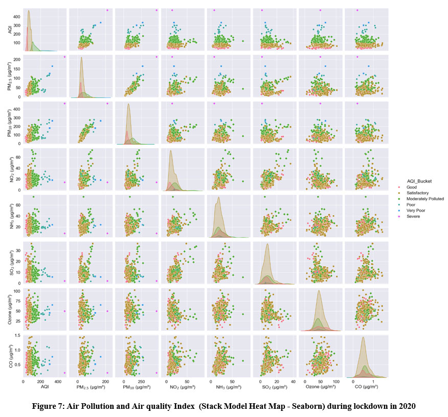Figure 7: Air Pollution and Air quality Index (Stack Model Heat Map - Seaborn) during lockdown in 2020. Click here to view Figure

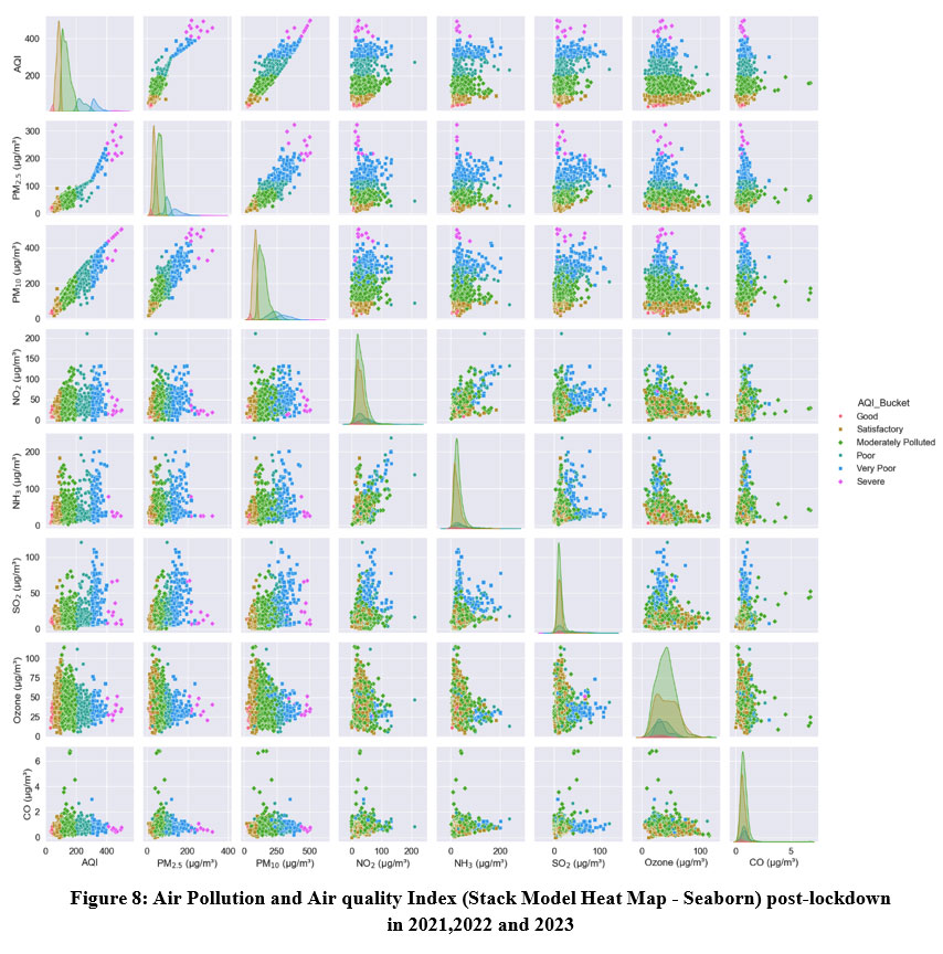Figure 8: Air Pollution and Air quality Index (Stack Model Heat Map - Seaborn) post-lockdown in 2021,2022 and 2023. Click here to view Figure

Correlation Matrix

The heat map in Figure 9 graphically illustrates the correlation between all of the attributes used in the air quality dataset. For every value to be plotted, a heatmap has values that represent different shades of the same hue. On a chart, higher values are typically represented by darker hues than lighter ones. Another option is to use an entirely different color for a very different value. The strength of the inter-correlations among the metrics implies that distinct air pollutants influence the AQI. Correlation refers to the mutual relationship between two variables. When one parameter's value increases or decreases, it has a direct correlation with the other. When one parameter rises and the other rises, there is a positive correlation and when one parameter increases and the other's value reduce, there is a negative correlation. The amount ranges from +1 to -1. The connection is considered strong when it falls between +0.8 and 1.0 and -0.8 and -1.0, and moderate between +0.5 and +0.8 and -0.5 and -0.8. The heatmap shows the correlation coefficient value between the parameters. When the correlation falls within these ranges, AQI is positively related to both PM_2.5 (0.90) and PM₁₀ (0.91). This demonstrates that PM₁₀ and PM_2.5 concentrations directly affect the AQI value. Strong negative correlations exist between the Ozone (O₃) (-0.15) and the AQI, as well as between NO₂ (-0.19) and both. The primary causes were shown by the quick decline in the ozone titration reaction, which led to a dramatic shift in the association between them at this stage and extremely low NO₂ .^27,28 This information is crucial for understanding the connection among air quality parameters and their impact on the overall AQI value. By analyzing these correlations, policymakers and researchers can better target interventions to improve air quality in specific areas.

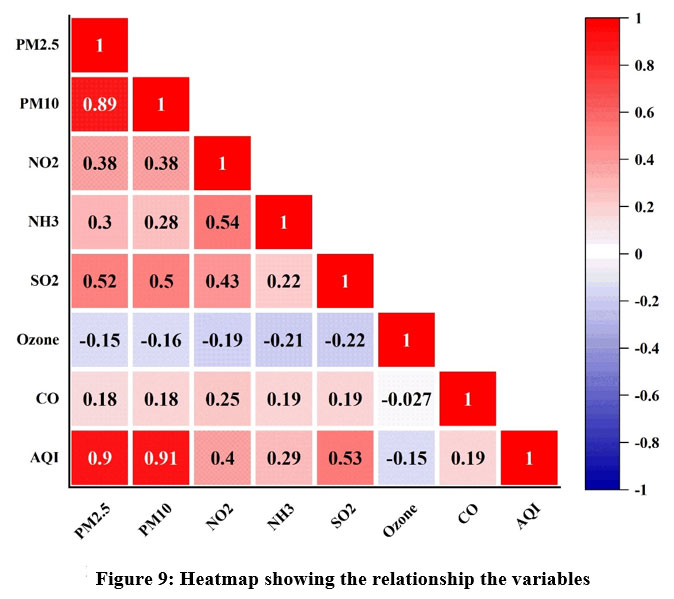Figure 9: Heatmap showing the relationship the variables. Click here to view Figure

Models Analysis

Model analysis was conducted for accuracy and prediction using Python programming. Using datasets obtained from CPCB website in Rajasthan, the data frame has a range index of 3680. This value was computed from the data.

This information is available on the CPCB, Government of India, official website. The authors standardized the data format and eliminated outliers and null values to preserve good data quality. After removing outliers, null values, and missing values, the dataset which included 3314 points was subjected to (LR), (DTR), (RFR) , (XGBoost)   and (KNN) analyses. After data preparation, Table 2 illustrates the summary statistics of the desired variable and the independent variables.

Table 2: Component descriptive statistics

During the analysis, normalize the data points before dividing the dataset for training and testing. We trained the models using 2651 data points (80%) and tested those using 662 data points (20%) out of a total of 3314 data points. The study used two measurements to check how well the model could predict.i.e., RMSE and R². These were based on the actual and predicted values.

Table 3: Dependent Air pollutants and Independent AQI Model’s Effectiveness

This study used models and metrics from CPCB data to evaluate the model's performance. Table 3 provides these metrics. Author conduct a comparative study for the appropriate five-year pre-lockdown (2019), lockdown (2020), and post-lockdown (2021–2023) periods of March, April, and May.

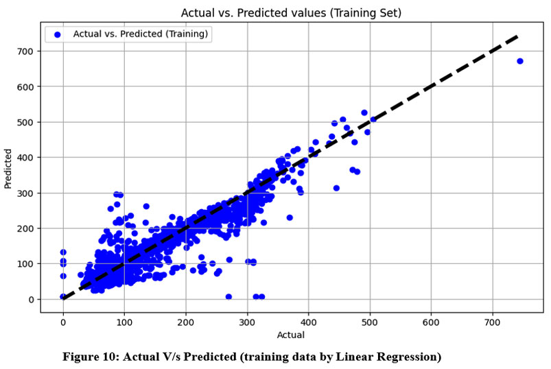Figure 10: Actual V/s Predicted (training data by Linear Regression) Click here to view Figure

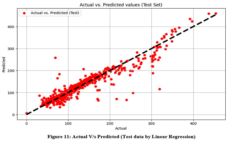Figure 11: Actual V/s Predicted (Test data by Linear Regression) Click here to view Figure

A linear regression analysis is depicted in Figures 10-11, where the independent variable is the AQI for model accuracy, and the dependent variable is an air pollutant. With a random state of 70, the data used comprised 80% training and 20% test data. The R² values for the training and testing datasets are closer to the straight line (0.86, 0.88) at their highest points, as observed in the graph between the actual AQI values and predicted values. We can infer that the model's R² value is closer to one, indicating its effectiveness in most cases and clear depiction of trends (86.00 to 88.00).

Figure 12: Actual V/s Predicted (training data by Decision Tree regression) Click here to view Figure

Figure 13: Actual V/s Predicted (Testing data by Decision Tree regression). Click here to view Figure

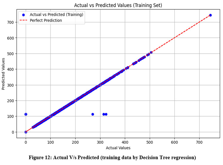
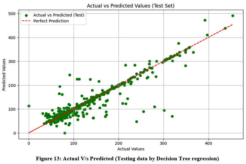
Figures 12–13 display the results of a decision tree regression study in which air pollutants are the experimental variable and the aqi is the manipulated variable used to measure the model's correctness. It utilized 80% of the data for training and 20% for testing, with a random state value of 70. The graph comparing the actual AQI to the predicted AQI for both training and testing data indicates that Decision Tree Regression (0.98, 0.83) yields the highest R² responses close to the straight line. This suggests that the model performs effectively in most cases and clearly depicts trends.

Figure 14: Actual V/s Predicted (training data by Random Forest Regression). Click here to view Figure

Figure 15: Actual V/s Predicted (Test data by Random Forest Regression). Click here to view Figure

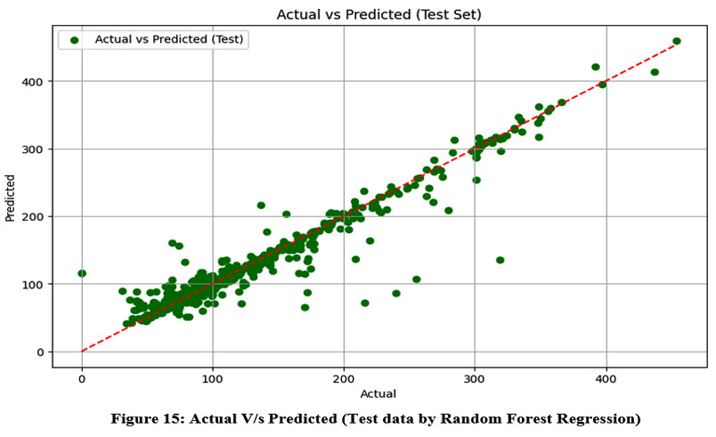
Figures 14–15 depict a random forest regression study with an air pollutant as the response variable and AQI as the explanatory variable for model validity. In this study, the author used a random state of 70. The maximum responses of R² for the training and testing datasets in random forest regression (0.97, 0.92) are closer to the straight line on the graph representing the actual versus predicted AQI. This shows that the model has an R² value closer to one, signifying its satisfactory performance in many cases and its ability to display trends nicely with adequate accuracy of the model (97.00, 92.00).

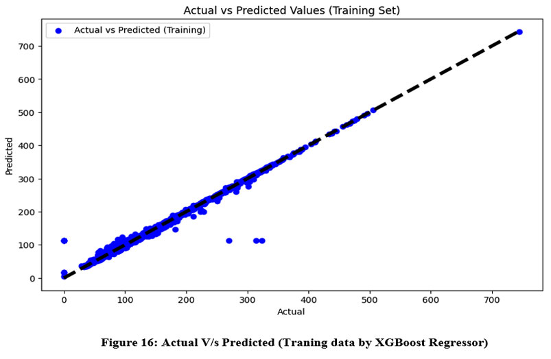Figure 16: Actual V/s Predicted (Traning data by XGBoost Regressor). Click here to view Figure

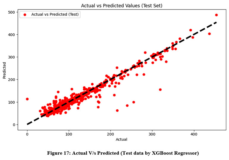Figure 17: Actual V/s Predicted (Test data by XGBoost Regressor) Click here to view Figure

Figures 16–17 depict an Extreme gradient boosting regressor study with an air pollutant and AQI for model validity. The maximum responses of R² for the training and testing datasets in random forest regression (0.98, 0.92) are closer to the straight line on the graph representing the actual versus predicted AQI for both datasets. This indicates that the model has an R² value closer to one, signifying its satisfactory performance in many cases and its ability to display trends nicely with adequate accuracy of the model (98.00, 92.00). The errors for linear regression (LR) are shown in Table 3, along with the root mean square error values for the train and test datasets (27.48 and 24.09, respectively). Similarly, the study obtain errors for Decision Tree Regression (DTR), which include RMSE values for both datasets (7.67, 28.19). In Addition, the study also get errors for Random Forest Regression (RFR), with RMSE values of 11.47 and 19.22 datasets, respectively. However, extreme gradient boosting (XGBoost) found that the minimum root mean square error for both datasets was 8.47 and 18.87.

In the study period, it was found that extreme gradient boosting regression analysis demonstrates superior performance compared to linear regression (86.00, 88.00), decision tree regression (98.00, 83.00), and random forest regression (97.00, 92.00) in terms of accuracy for both the training and testing datasets (98.00, 92.00). Therefore, we consider it a suitable framework for evaluating the accuracy of Rajasthan's air quality, as it shows minimal RMSE errors without any instances of under- or over-fitting.

Table 4: Dependent Air pollutants and Independent AQI_Bucket Model’s Effectiveness

The training and testing accuracies of each classifier are provided in Table 4. The Extreme gradient boosting and the Random Forest Classifier are achieved the best results across all datasets, with scores of 99% in the training data and (92.00 , 93.00) in the testing data respectively. Conversely, the logistic classifier yielded training and testing scores of 66% respectively, predicting the worst outcomes. Additionally, KNN classifiers obtained 92% accuracy in the training dataset and 86% in the testing dataset and Decision tree classifier found 99% training data with 89% of testing datasets . The best-performing classifier among the five datasets in Table 4 is the Extreme gradient boosting Classifier. Furthermore, we observe that AQI accuracy and prediction results are satisfactory when feature selection is utilized.

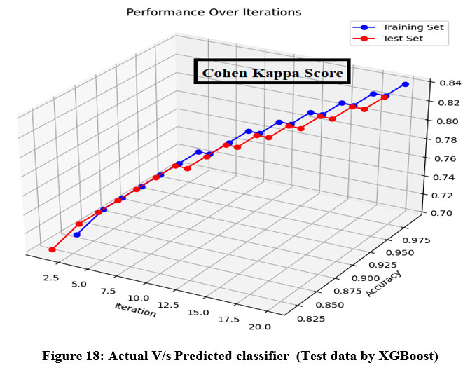Figure 18: Actual V/s Predicted classifier (Test data by XGBoost) Click here to view Figure

The actual vs. predicted classifier is depicted in Figure 18. The highest Kappa score for random forest regression during the study period was 0.89. As a result, Extreme gradient boosting emerges as the most effective model for predicting AQI.

Conclusion

The following conclusions have been reached from the overall results and discussion:

Alwar exhibited the largest percentage deduction in AQI whereas Jodhpur had the lowest reduction among the mentioned location during Pre-lockdown and Lockdown period.

According to the study's findings, which utilized Pearson correlation analysis, there is a significant relationship between AQI and PM levels. However, there was only an insignificant connection among the Air Quality Index (AQI) and Ozone .

Extreme gradient boosting got accuracy scores of 98.00% for the training dataset and 92.00% for the testing dataset. This is much higher than the 86.00% and 88.00% for linear regression, 98.00% and 83.00% for decision tree regression, and 97.00% and 92.00% for random forest regressors.

In this study period, the model found a maximum kappa score of 0.89 for the air quality index (AQI) model prediction using an extreme gradient boost.

Acknowledgment

We thank the Central Pollution Control Board (India) for providing the data for this study.

Funding source

The authors did not received support from any agency for this study or research work

Conflict of Interest

The authors declare that they have no known competing financial interests or personal relationships that could have appeared to influence the work reported in this paper.

Authors’ Contribution statement

Mr. Vikram Singh Bhati: Writing original draft; Writing - review & editing; Figure preparation; Formal analysis.

Dr. Abhishek Saxena: Conceptualization; Investigation; Methodology; Software; Writing original draft

Dr. Ravi Khatwal: English Writeup, Logical thinking

Data Availability Statement

Data available publicly at https://airquality.cpcb.gov.in/ccr/#/caaqm-dashboard-all/caaqm-landing

Ethics Approval Statement

NIL

Reference

1. Liu H, Li Q, Yu D, Gu Y. Air quality index and air pollutant concentration prediction based on machine learning algorithms. Appl Sci. 2019;9(19):4069.
   CrossRef
2. Sahoo PK, Mangla S, Pathak AK, Salãmao GN, Sarkar D. Pre-to-post lockdown impact on air quality and the role of environmental factors in spreading the COVID-19 cases: a study from a worst-hit state of India. Int J Biometeorol. 2021; 65:205-222.
   CrossRef
3. Mahato S, Talukdar S, Pal S, Debanshi S. How far climatic parameters associated with air quality induced risk state (AQiRS) during COVID-19 persuaded lockdown in India. Environ Pollut. 2021; 280:116975.
   CrossRef
4. Guttikunda SK, Dammalapati SK, Pradhan G, Krishna B, Jethva HT, Jawahar P. What is polluting Delhi’s air? A review from 1990 to 2022. Sustainability. 2023;15(5):4209.
   CrossRef
5. Suroshe S, Dharpal SV, Ingole NW. Prediction of air quality index using regression models. GIS Sci J. 2022;9(8):576-591.
6. Julfikar SK, Ahamed S, Rehena Z. Air quality prediction using regression models. In Applications of Artificial Intelligence and Machine Learning. ICAAAIML 2020; 2021:251-262.
   CrossRef
7. Ikhlasse H, Benjamin D, Vincent C, Hicham M. Environmental impacts of pre/during and post-lockdown periods on prominent air pollutants in France. Environ Dev Sustain. 2021;23(9):14140-14161.
   CrossRef
8. Xu Y, Liu X, Cao X, et al. Artificial intelligence: A powerful paradigm for scientific research. The Innovation. 2021;2(4).
   CrossRef
9. Goodfellow I, Bengio Y, Courville A. Deep Learning. MIT Press; 2016.
10. Saravanan R, Sujatha P. A state of art techniques on machine learning algorithms: a perspective of supervised learning approaches in data classification. In 2018 Second International Conference on Intelligent Computing and Control Systems (ICICCS). IEEE; 2018:945-949.
    CrossRef
11. Hope TM. Linear regression. In Machine Learning. Academic Press; 2020:67-81.
    CrossRef
12. Ravindiran G, Hayder G, Kanagarathinam K, Alagumalai A, Sonne C. Air quality prediction by machine learning models: a predictive study on the Indian coastal city of Visakhapatnam. Chemosphere. 2023; 338:139518.
    CrossRef
13. Sunku VSRP, Mukkamala R, Namboodiri V. Air quality index prediction using multivariate deep neural networks: a case study of a proposed state capital in India. Journal of Air Pollution and Health. 2023;8(3).
    CrossRef
14. Jung CR, Hwang BF, Chen WT. Incorporating long-term satellite-based aerosol optical depth, localized land use data, and meteorological variables to estimate ground-level PM2.5 concentrations in Taiwan from 2005 to 2015. Environmental Pollution. 2018; 237:1000-1010.
    CrossRef
15. Harishkumar KS, Yogesh KM, Gad I. Forecasting air pollution particulate matter (PM2.5) using machine learning regression models. Procedia Computer Science. 2020; 171:2057-2066.
    CrossRef
16. Kumari S, Lakhani A, Kumari KM. COVID-19 and air pollution in Indian cities: world’s most polluted cities. Aerosol and Air Quality Research. 2020;20(12):2592-2603.
    CrossRef
17. Patil RM, Dinde HT, Powar SK, Ganeshkhind PM. A literature review on prediction of air quality index and forecasting ambient air pollutants using machine learning algorithms. Int J Innov Sci Res Technol. 2020;5(8):1148-1152.
    CrossRef
18. Bhalgat P, Pitale S, Bhoite S. Air quality prediction using machine learning algorithms. International Journal of Computer Applications Technology and Research. 2019;8(9):367-370.
    CrossRef
19. Bellinger C, Mohomed Jabbar MS, Zaïane O, Osornio-Vargas A. A systematic review of data mining and machine learning for air pollution epidemiology. BMC Public Health. 2017; 17:1-19.
    CrossRef
20. Yadav R, Vyas P, Kumar P, Sahu LK, Pandya U, Tripathi N, Gupta M, Singh V, Dave PN, Rathore DS, Beig G. Particulate matter pollution in urban cities of India during unusually restricted anthropogenic activities. Frontiers in Sustainable Cities. 2022; 4:792507.
    CrossRef
21. Ruhela M, Maheshwari V, Ahamad F, Kamboj V. Air quality assessment of Jaipur city Rajasthan after the COVID-19 lockdown. Spatial Information Research. 2022;30(5):597-605.
    CrossRef
22. Pacheco H, Díaz-López S, Jarre E, Pacheco H, Méndez W, Zamora-Ledezma E. NO2 levels after the COVID-19 lockdown in Ecuador: a trade-off between environment and human health. Urban Climate. 2020; 34:100674.
    CrossRef
23. Menut L, Bessagnet B, Siour G, Mailler S, Pennel R, Cholakian A. Impact of lockdown measures to combat Covid-19 on air quality over western Europe. Science of the Total Environment. 2020; 741:140426.
    CrossRef
24. Chen LWA, Chien LC, Li Y, Lin G. Nonuniform impacts of COVID-19 lockdown on air quality over the United States. Science of the Total Environment. 2020; 745:141105.
    CrossRef
25. Pei Z, Han G, Ma X, Su H, Gong W. Response of major air pollutants to COVID-19 lockdowns in China. Science of the Total Environment. 2020; 743:140879.
    CrossRef
26. Nakada LYK, COVID RU. Pandemic: impacts on the air quality during the partial lockdown in São Paulo state, Brazil. Science of the Total Environment. 2020; 730:139087.
    CrossRef
27. Pusede SE, Steiner AL, Cohen RC. Temperature and Recent Trends in the Chemistry of Continental Surface Ozone. Chem Rev. 2015;115(10):3898-3918.
    CrossRef
28. Wang L, Wang J, Fang C. Assessing the impact of lockdown on atmospheric ozone pollution amid the first half of 2020 in Shenyang, China. International Journal of Environmental Research and Public Health. 2020;17(23):9004.
    CrossRef
29. Taghinezhad E, Kaveh M, Szumny A, Figiel A. Quantifying of the best model for prediction of greenhouse gas emission, quality, and thermal property values during drying using RSM (Case Study: Carrot). Applied Sciences. 2023;13(15):8
    CrossRef
30. Sahu LK. Volatile organic compounds and their measurements in the troposphere. Curr Sci. 2012;102(11):1645-1649.
31. Lefohn AS, Wernli H, Shadwick D, Limbach S, Oltmans SJ, Shapiro M. The importance of stratospheric–tropospheric transport in affecting surface ozone concentrations in the western and northern tier of the United States. Atmos Environ. 2011;45(28):4845-4857
    CrossRef