Time Series Land Surface Temperature Induced Heat Stress Vulnerability in Tropical Cities: A Case Study from India
Aswathy Asok1
 , Sabu Joseph1
*
, Asok Laila Achu2
, Jobin Thomas3
and Girish Gopinath3
, Sabu Joseph1
*
, Asok Laila Achu2
, Jobin Thomas3
and Girish Gopinath3
1
Department of Environmental Sciences,
University of Kerala,
Thiruvananthapuram,
Kerala
India
2
Department of Climate Variability and Aquatic Ecosystems,
Kerala University of Fisheries and Ocean Studies (KUFOS),
Kochi,
Kerala
India
3
Department of Geology and Geological Engineering,
University of Mississippi,
Oxford,
MS
USA
http://dx.doi.org/10.12944/CWE.21.1.26
Copy the following to cite this article:
Asok A, Joseph S, Achu A. L, Thomas J, Gopinath G. Time Series Land Surface Temperature Induced Heat Stress Vulnerability in Tropical Cities: A Case Study from India. Curr World Environ 2026;21(1). DOI:http://dx.doi.org/10.12944/CWE.21.1.26
Copy the following to cite this URL:
Asok A, Joseph S, Achu A. L, Thomas J, Gopinath G. Time Series Land Surface Temperature Induced Heat Stress Vulnerability in Tropical Cities: A Case Study from India. Curr World Environ 2026;21(1).
Download article (pdf)
Citation Manager
Publish History

Introduction
Globally, urbanized areas cover about 3% of the total land area, yet about 55% of the world population resides in urban areas, which was only 30% back in 1950.1 While the urban areas serve as a hub for increased productivity, fostering economic growth and human development, the urbanization process poses significant challenges due to the modification of urban morphology. Tremendous social, economic and environmental impacts are caused as a result of global urbanisation. The global climate is also affected by urban expansion. 5% of the total emissions from tropical deforestation and land use change is predicted to contribute to the direct loss of vegetation from areas of high urban expansion.2 Between 1960 and 2019, LULC alterations have impacted approximately one-third of the global land surface.3 The transformation of naturally vegetated areas into impervious surfaces results in suboptimal land use/ land cover (LULC) pattern, which increases the occurance and intensity of extreme rainfall events as well as heat stress in urbanized regions.4
Increase in the land surface temperature (LST) and change in evaporation rates due to urbanization affects the natural variability of heating and cooling rates between the urban areas and neighbouring peri-urban/rural areas. Urban heat island (UHI) is one of the critical outcomes of the differential cooling rates, forming substantially warmer urban areas than surrounding suburban and rural counterparts.5 The UHI effect within an urban area has been found to be correlated with vegetation and building characteristics.6,7
The most reliable estimate of the human - induced increase in temperatures from 1850-1900 to 2010-2019 is approximately 1.1°C. These changes encompass heightened occurrences of drought, floods and other extreme natural phenomenoa.8 Understanding the evolution of urbanization pattern and LULC changes remain a crucial component to be considered in sustainable urban planning and environmental management. Similarly, LST patterns furnish valuable insights into urban microclimates, thereby facilitating an enhanced comprehension of UHI dynamics.9,10
Recognizing the significant effects of LULC changes in urbanized areas on UHIs, numerous studies have been carried out in different urban settings worldwide to examine the spatial patterns of UHI and their impacts on the urban environment.11 In India as well, a large number of studies have addressed the impacts of urbanization and LULC changes on LST patterns and UHIs over large metropolitan cities, such as Delhi, Mumbai, Kolkata, Chennai, Jaipur, Nagpur, Hyderabad.12
In fast urbanizing places like Kochi, Kerala, urban heat islands (UHIs) are a major concern.13 Population density, land management techniques, and impermeable surfaces are some of the elements that aggravate the urban heat island (UHI) effect, which causes urban regions to experience warmer temperatures than their rural surrounds.14 According to studies, UHIs can have negative consequences on people's health and comfort, including higher levels of air pollution, greater heat stress on citizens, and damaged human health.15 UHI is a significant phenomenon that can lead to a vicious cycle in which energy-intensive cooling techniques exacerbate temperature increases.16 Furthermore, research has demonstrated how green areas might mitigate UHIs by lowering solar radiation input and lowering temperatures through shade and transpiration.17 The average temperature in cities is two to three degrees Celsius higher than that of their environs (56) Several studies have addressed the effects of changes in LULC in relation to LST and UHI18-19; But the subjection to heat stress index is not much considered. The present study on HSVI helps to identify the heat stress regions in the study area and helps to take up appropriate sustainable development policies.
The present study aims to (i) assess LULC conversions from 1988 to 2023 in a rapidly developing city (Kochi, India), (ii) interpret the interaction between time series LST and spectral indices such as NDBI and NDVI, (iii) investigate the UHI effects in Kochi city, and (iv) propose a Heat Stress Vulnerability Index (HSVI) using the AHP method for promoting sustainable urban development.
Study Area
the present study was carried out in Kochi, one of the biggest urban centers in Kerala (India) (Fig. 1). The Kochi city region has an area of 94.88km2. In this study, we used a 10 km buffer from the centre of the Kochi city region (i.e., between 9° 46’18” N to 9° 49’49” N latitude and 76° 17’ 24” E to 76° 49’ 9” E longitude), covering an area of 666km2 to understand the LULC changes and variations in LST across the region (Fig.1). Kochi is interlaced by the Vembanadu wetland system on the southwest coast of Kerala and the urbanized zone is mostly developed along the shores of the Vembanadu estuary. Being developed largely on the coastal plain and lowland physiographic zone of Kerala, the maximum elevation of the region reaches up to 8.73 feet above the mean sea level, with the urban landscape gently sloping from east to west. The western part of the urbanized zone is characterized by its flat terrain and is interspersed by a network of canals connecting seamlessly to the Vembanadu lagoon. Kochi is connected to other parts of the country by all means of transportation. The major national highways passing through the urban zone are NH85, NH66, NH544, NH966B, etc., allowing the majority of the commercial traffic. Kochi is linked to other places in the country through major railway lines. Kochi also has a strong system of inland waterways made up of rivers, canals, and backwaters.
Kochi is an Urban Agglomeration (UA) in the Million Plus UA category, with a population of 3,193,000 in 2021-2022, according to estimates from the last Census. Over the past ten years, Kochi City's population has grown by 5.6% (1991-2001).20 The city’s economic growth began with the reforms brought by the Central government in 1990. The economy was boosted by the service sector, with the establishment of IT park and port-based constructions.21 Being the commercial hub of Kerala, Kochi serves as a pivotal regional economic center, hosting several electronics/information technology-based companies and related sectors.22 Maritime activities also play a central role in the regional economy, with Kochi being recognized as one of the 12 major seaports in India (GoI, 2019). The region holds one of the largest international container transshipment terminals in India. Kochi also houses other significant marine facilities, such as the Southern Naval Command of the Indian Navy, the State Headquarters of the Indian Coast Guard, the Cochin Shipyard, the Port of Kochi, Cochin Special Economic Zone, etc. The Cochin Special Economic Zone (CSEZ) was established in September 1983 by the Department of Commerce, Government of India. The zone is one of the seven government-owned zones located in Kakkand.21
The climate in Kochi is tropical. The temperature fluctuates between 26 and 33 °C each year. Because of its proximity to the sea and extensive interior water bodies, the humidity is high throughout the year.21-26 The region is characterized by different local climate zones based on the variations in building morphology, street width, vegetative fraction, sky view factor, and anthropogenic heat flux.22,23 The dominant local climate zones include open low-rise, compact low-rise, compact midrise and open high-rise with varying impervious surface fractions and distinct meteorological conditions.24,25
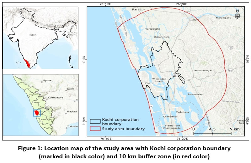 | Figure 1: Location map of the study area with Kochi corporation boundary (marked in black color) and 10 km buffer zone (in red color).
|
Materials and Methods
The present study utilized a methodology integrating multi-temporal remote sensing data (Landsat 5-TM, Landsat 7 ETM+, and Landsat 8 OLI) with the AHP technique to understand the changes in LULC and LST over the region and to develop the HSVI. We also used the gridded population density data (gpw-v4-population-density-rev11) from the Socio-Economic Data and Applications Center (SEDAC) for obtaining HSVI.
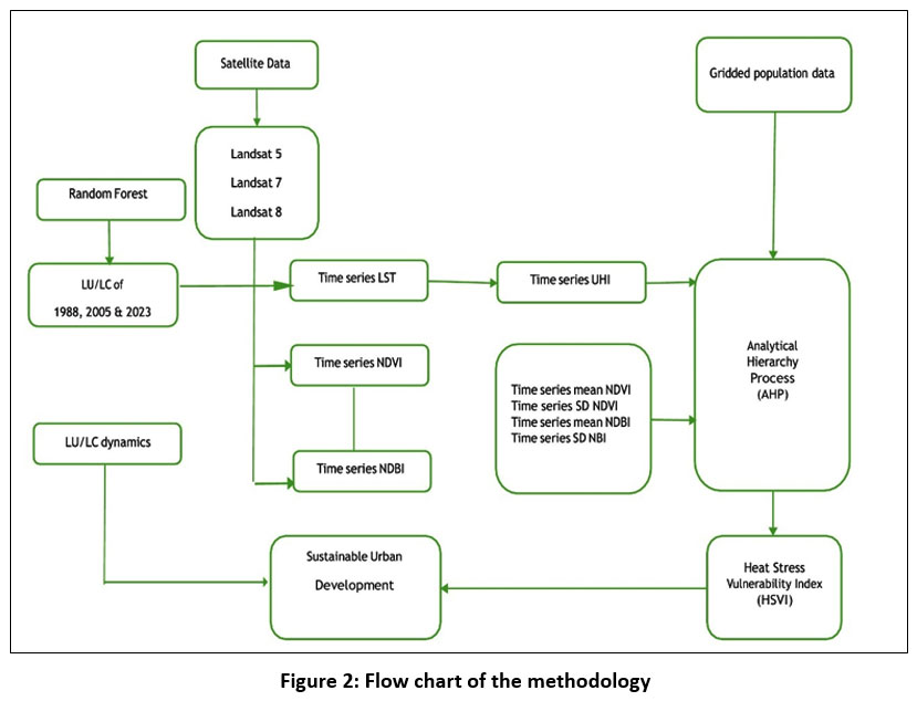 | Figure 2: Flow chart of the methodology
|
Land Use / Land Cover Classification
We used the Random Forest (RF)27 classification method to classify LU/LC from satellite images for the years 1988, 2005, and 2023. From the time series satellite data, only 3 years were used for the LU/LC classification. The RF classifier comprises a combination of tree classifiers, where each classifier is created using a random vector independently sampled from the input training data. A method used to generate a training dataset by randomly drawing with replacement N pixels, called bagging, was employed for each feature.28 Pixels were classified by selecting the class that received the most votes from all the tree predictors. The selection of an attribute selection method is essential for the design of a decision tree. The choice of an attribute selection method is necessary for the design of a decision tree. A number of approaches are available for selecting attributes, the majority of which assign a quality measure directly to the attribute. The most commonly used attribute selection measure in the design of decision trees is the Gini Index29 and hence it is utilized in this study. When randomly selecting one case (pixel) from a specified training set (T) and assigning it to a particular class Ci, the Gini index is expressed as:
![]()
where f (Ci, T)/|T| is the probability that the selected case belongs to class Ci. The prime factors for choosing Random Forest (RF) as the classification technique in this study include: a) its effectiveness with input predictors of varied nature, b) the capability to obtain a measure of variable importance, which is useful for feature selection in multi-source data classification, and c) its robustness to noise and outliers.30
Accuracy assessment
Three different error metrics were used in this study to assess the accuracy of the LU/LC classification. One of the important measures of accuracy assessment is the Cohen31 The Kappa index (K) assesses the concordance between observed and expected data. In addition, the post classification accuracy was examined using measures, such as the producer’s accuracy, user’s accuracy, and overall accuracy, which is calculated using the given equations.
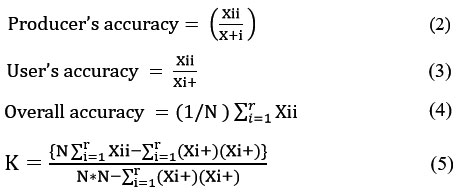
where N indicates the entire number of pixels used in classification, Xii represents the count of pixels that are correctly classified in row (r) and column (i), Xi+ and X+i are the total number of samples in column (i) and row (r) in the matrix.
Spectral Indices
We used the spectral indices, viz., Normalized Difference Vegetation Index (NDVI) and Normalized Difference Built-up Index (NDBI), to derive the relationship between LST and LU/LC of the region. The derivation of NDVI (Eq. 6) utilizes the visible red and near-infrared (NIR) wavelengths.32 The values of NDVI typically range from +1.0 to -1.0, with negative values indicating clouds and water, positive values (< 0.30) indicating bare soil, and positive values of NDVI (> 0.60) implying dense green vegetation.
Eq(6)
![]()
The NDBI is a spectral index commonly used to evaluate the impervious surface or built-up area in a region.33 Its derivation uses the NIR and short-wave infrared (SWIR), and the index ranges from +1.0 to -1.0 (Eq. 7).
![]()
We used the NDVI to establish the relationship between LST and vegetated areas, and the NDBI to derive the relationship between LST and built-up areas.
Land Surface Temperature (LST)
An important geophysical measure of the land-atmosphere system's surface energy and water balance is the LST. To extract LST from space-based thermal infrared (TIR) data, several approaches have been developed. Techniques of LST estimation consist of the following steps: (1) Obtaining spectral radiance from DN values, (2) deriving Brightness temperature, (3) Calculating land surface emissivity, and (4) Assessment of brightness temperature to LST and producing Degree Celsius value of LST.
Equation 8 is used to obtain the spectral radiance of the thermal band of Landsat 5 TM and Landsat 7 ETM+
![]()
Where, QCAL represents Quantized calibrated pixel value in DN; QCALMIN & QCALMAX denote minimum and maximum quantized calibrated pixel value in DN; LMINh and LMAXh Spectral radiance scaled to QCal Max Ns QCal Min.
For Landsat 8 OLI, the spectral radiance is estimated by equation 9
![]()
![]()
Where BT is the brightness temperature in Kelvin, E is the Land surface emissivity.
Land surface emissivity is a proportion of vegetation, which is calculated using equation 11.
![]()
Where PV can be calculated by equation 12.32
![]()
UHI Estimation
The UHI is estimated as Eq. 13,
![]()
Where LST is the estimated land surface temperature, LST mean is the mean LST, and SD represents the standard deviation.34
Heat Stress Vulnerability Index
In this study, we derived the HSVI using temporal LST variation, LULC, proximity from the green space and population density. Temporally averaged LST (LST Mean) for a period of 10 years was estimated using LST between 2014 and 2023. Proximity from the green space was obtained from the LULC map of 2023 using Euclidean Distance method, Mean of NDBI (NDBI mean) and mean of NDVI (NDVI mean) for the years 2014 to 2023 were also calculated. Demographic details of the study area were extracted from SEDAC. We made use of the gridded population density data (gpw-v4-population-density-rev11). The Analytical Hierarchy Process (AHP) technique, which is frequently employed in multi-criteria decision analysis (MCDA) for the examination of complicated situations, estimates the relevance of the input components.36 The relative importance of factors and sub-classes was estimated by the AHP technique, which is widely used in multi-criteria decision analysis (MCDA) for analysing complex decision-making problems.35 A comparison matrix was developed by assessing the importance of various heat stress influencing factors.34
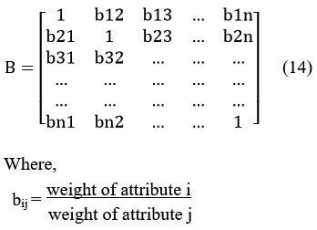
The Eigen values were estimated after computing the relative weightage of each factor, and corresponding normalized Eigen vectors (NEV) were also estimated. The consistency ratio (CR) was used to determine the consistency related to the pairwise comparison matrix.
![]()
in which the consistency Index (CI) was calculated using Eq. 16, where RI is the consistency index of a random square matrix of the same order.
![]()
Where h max is the largest Eigen value of “B” and n is the order of the square matrix.
CI value will be zero if B becomes perfectly consistent.36 Commission and omission of a factor rely on the CR value, where the factors with a CR value>0.1 were omitted from further analysis. ArcGIS was used to derive HSVI using the equation 17.
![]()
where Wj is the weightage of the influencing factor “j,” Wij is the weightage of the class “i” of the factor “j.”
One of the limitations of the method is that there may not be a strong correlation between the HSVI and heat-related health outcomes; hence, additional validation of the HSVI should be carried out in different places to confirm the index's dependability. Furthermore, the location and duration of validation data are crucial for improving HSVI's dependability.
Results and Discussion
Land Use Land Cover Dynamics
The LU/LC pattern over the analysed period (1988-2023) is depicted in Fig 3, and Table 1 provides the areal coverage for each LU/LC type during the period. Notably, the period from 2005 to 2023 marked the most pronounced changes, with a 6.25% increase compared to the more modest increase of 3.5% observed between 1988 and 2005. In 1988, urban settlements accounted only for < 10% of the total area, which increased to 19% by 2023, that is over a period of 35 years, from 1988 to 2023, the area under built-up has increased by about 10%. This increase in built-up area is related to the increase in land surface temperature. There has been a decrease in vegetation over the period of study from 52.97% to 42.19%, which also adds up to the increase in temperature. The area under agriculture shows fluctuations from 1988 to 2023, that is, it shows a 10.8% increase in 2005 from 1988 and 3.68% decrease in 2023. This decrease in agriculture area also leads to an increase in LST. In 1988, barren land decreased from 9% to 6% during 1988 to 2023. This phenomenon is likely to be associated with the expansion of urban areas encroaching upon previously barren lands. The spatial extent of waterbodies experienced fluctuation from 1988 to 2005, initially covering 20% of the total area, increasing to around 23% by 2005, and subsequently declining to 21% by 2023.
The classified LU/LC maps are validated using Kappa index, User's accuracy, Producer's accuracy and overall accuracy (OA). Table 2 shows that the LULC map of 1988 attained an overall accuracy of 92.5% and Kappa value (K-value) of 90.4, indicative of satisfactory performance. User's accuracy for the 1988 map varied from 81.2 to 100%, while producer's accuracy was highest for waterbodies (100%) and lowest for vegetation (87.5%). Commission and omission errors for the 1988 map ranged from 0 to 18.75 and 0 to 13.63, respectively.
In the case of the 2005 LU/LC, an overall accuracy of 90.5% with a Kappa value of 88.18 is reported, indicating good accuracy (Table 3). The highest user's accuracy was observed in the water body category (100%), while the lowest was in agriculture (81.8%). Water bodies and built-up areas exhibited maximum producer's accuracy (100%), whereas vegetation showed the lowest (76.2%). Commission and omission errors for the 2005 map ranged from 0 to 18.18 and 0 to 18.51, respectively.
Similarly, the LU/LC map of 2023 demonstrated an overall accuracy of 94.1 and a K-value of 92.61 (Table 4). In this map, the highest user's accuracy was associated with the water body category (100%), while the lowest was in open areas (81.25%). Producer's accuracy indicated higher accuracy for waterbodies and lower accuracy for vegetation. Commission and omission errors for the 2023 map ranged from 0 to 0.13 and 0 to 18.51, respectively. Overall, all three LULC maps exhibited overall accuracies exceeding 80%, signifying excellent agreement.38,39
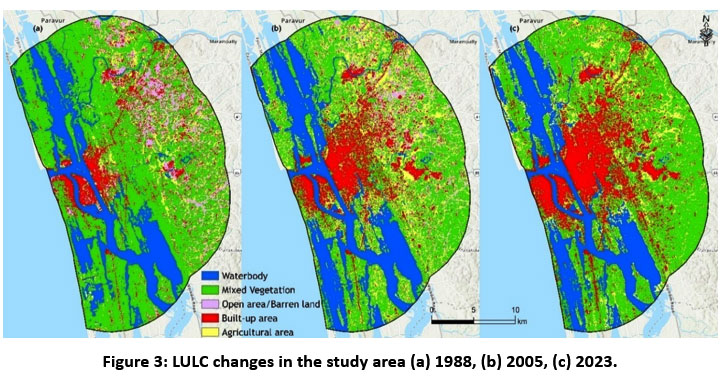 | Figure 3: LULC changes in the study area (a) 1988, (b) 2005, (c) 2023.
|
Table 1: LULC changes in the study area from 1988 to 2023.
1988 | 2005 | 2023 | ||||
LULC Class | Area (Km2) | Area (%) | Area (Km2) | Area (%) | Area (Km2) | Area (%) |
Waterbody | 136 | 20.45 | 158 | 23.83 | 146 | 21.92 |
Built-up area | 63 | 9.47 | 86 | 12.97 | 128 | 19.22 |
Open area/Barren land | 61 | 9.17 | 44 | 6.64 | 10 | 1.50 |
Mixed Vegetation | 352 | 52.93 | 250 | 37.71 | 281 | 42.19 |
Agricultural area | 53 | 7.97 | 125 | 18.85 | 101 | 15.17 |
Table 2: Accuracy assessment of LULC in 1988
Waterbody | Vegetation | Built-up | Open | Agriculture | Total | Commission | User's | |
Waterbody | 33 | 33 | 0 | 100 | ||||
Vegetation | 28 | 1 | 1 | 30 | 6.6 | 93.33 | ||
Built-up | 1 | 19 | 1 | 21 | 9.5 | 90.47 | ||
Open area | 1 | 1 | 18 | 20 | 10 | 90 | ||
Agriculture | 2 | 1 | 13 | 16 | 18.75 | 81.25 | ||
Total | 33 | 32 | 22 | 20 | 13 | 120 | ||
Error: Omission (%) | 0 | 12.5 | 13.63 | 10 | 0 | Overall accuracy: 92.5% | ||
Table 3: Accuracy assessment of LULC in 2005
Waterbody | Vegetation | Built-up | Open | Agriculture | Total | Commission | User's accuracy | |
Waterbody | 22 | 22 | 0 | 100 | ||||
Vegetation | 24 | 2 | 26 | 7.69 | 90.3 | |||
Built-up | 3 | 26 | 29 | 10.3 | 89.65 | |||
Open area | 1 | 1 | 16 | 18 | 11.1 | 88.88 | ||
Agriculture | 1 | 3 | 18 | 22 | 18.18 | 81.81 | ||
Total | 22 | 29 | 27 | 21 | 18 | 117 | ||
Error: Omission | 0 | 17.24 | 3.7 | 18.51 | 0 | Overall accuracy: 90.59 | ||
Producer's accuracy | 100 | 76.19 | 96.29 | 100 | 82.75 | Kappa index: 88.18 | ||
Table 4: Accuracy assessment of LULC in 2023
Waterbody | Vegetation | Built-up | Open | Agriculture | Total | Commission | User's | |
Waterbody | 31 | 31 | 0 | 100 | ||||
Vegetation | 19 | 1 | 20 | 0.05 | 86.25 | |||
Built-up | 1 | 27 | 2 | 30 | 0.1 | 96.42 | ||
Open area | 1 | 1 | 13 | 15 | 0.13 | 81.25 | ||
Agriculture | 1 | 23 | 24 | 0.041 | 95.83 | |||
Total | 31 | 22 | 28 | 16 | 23 | 120 | ||
Error: Omission | 0 | 17.24 | 3.7 | 18.51 | 0 | Overall accuracy: 94.16% | ||
Producer's accuracy | 100 | 76.19 | 96.29 | 81.25 | 100 | Kappa index: 92.61% | ||
The longitudinal analysis of LULC maps spanning 35 years reveals a discernible trend wherein the built-up area experienced a notable increase of 9.48%, contrasting with declines in other classes such as vegetation (-10.74%) and open area (-7.01%). This trend can be attributed to various factors, with population growth and infrastructure development emerging as primary contributors.40
Analysis of Spectral Indices
The present study employs two key spectral indices, viz., the Normalized Difference Vegetation Index (NDVI) and the Normalized Difference Built-Up Index (NDBI), averaged over the ten-year period from 2014 to 2023. NDVI is widely recognized for its utility in assessing vegetation dynamics globally, with its time series exhibiting considerable inter-annual variability and diverse evolutions influenced by factors such as location, scale, and temporal period.41 NDVI maps the presence of vegetation, or the quantity or state of vegetation, on a pixel-by-pixel basis. The mean value of NDVI in the study area ranges from 0.49 to -0.10 (Fig 3). It is evident from the figure that the high NDVI shows high values for vegetation and water body and low values for built-up and barren areas. Moreover, there is an indirect relationship between NDVI and LST, which means that when NDVI increases, LST decreases.
In contrast, NDBI, an enhanced algorithm for detecting built-up areas, has gained prominence for its efficacy in delineating urban regions. Its mean values in the study area range from 0.20 to -0.36, with higher values indicating built-up presence and lower values suggestive of vegetation.41,42 Notably, core areas within the study site exhibit ascending NDBI values accompanied by a rapid decline in NDVI values. Higher the NDBI values, higher will be the LST value for that area. This dynamic is attributed primarily to vegetation-built-up trade-offs, highlighting the intricate interplay between land cover categories.
Spatial Variations of LST over the study area
Thermal band of the Landsat images were used to calculate the LST of the study area for the years 2014 to 2023. The mean LST values are shown in Fig. 4. During 2014, the higher and lower values of LST were 35.33 and 17.43oC, respectively. This increased to 40.45 and 24.50oC in 2023. Over the period of study from 2014 to 2023, the values of LST kept fluctuating around the mean high value of 37.73 and the low value of 25.93.
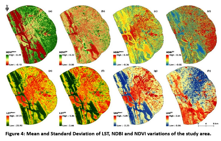 | Figure 4: Mean and Standard Deviation of LST, NDBI and NDVI variations of the study area.
|
Based on the LST maps, it is evident that LST values exhibit a dispersion pattern extending from the central region towards the eastern sector of the research area. This locale is characterized by pronounced urban expansion during the study period. The LULC change analysis indicates a substantial conversion of vegetation, open spaces, and water bodies into built-up areas.
Table 5 illustrates that the mean LST values exhibit minimal variation for water bodies and vegetation, whereas a notable increase is observed in the LST values for built-up areas, rising from 27.89 to 30.03°C. Comparable temperature increases have been documented in various locations, including a 3.9°C rise in temperature reported in Upper-Hill, Nairobi, Kenya, between 2015 and 2017,48 a 2.99°C increase observed in Jaipur city from 2000 to 2011,49 and 8.9–10.3°C temperature rises over Mumbai, Nagpur, and Hyderabad.
Table 5: Mean LST values of different LULC classes over the years.
LULC class | 1988 | 2005 | 2023 |
Water Body | 25.88 | 24.75 | 26.49 |
Vegetation | 26.89 | 26.46 | 28.84 |
Agriculture | 26.85 | 27.29 | 28.78 |
Built up | 28.42 | 28.04 | 30.03 |
Others | 27.89 | 27.00 | 29.9 |
Correlation among LST, NDVI and NDBI in the study area
Fig 5 depicts the result of regression analysis between LST – NDVI and LST - NDBI. A total of 1000 random points were generated for the correlation analysis. NDVI demonstrates a robust negative correlation with LST, indicated by an R2 of 0.25 and a Pearson correlation coefficient of -0.50. This suggests that regions with lower NDVI values exhibit higher land surface temperatures, while areas with higher NDVI values tend to have lower land surface temperatures. Conversely, NDBI displays a strong positive correlation with LST, with an R2 value of 0.50 and a Pearson correlation coefficient of 0.75.
.jpg) | Figur 5: Correlation between mean LST, mean NDVI and mean NDBI
|
Spatial variation of the UHI effect
The UHI in Kochi was generated from the Land Surface Temperature. According to the analysis spatial distribution of UHI for the period of study ranges from 5.85 to -2.25 (Fig 5). It is evident that UHI is distributed over those regions of the study area that have high built-up intensity. UHI zones mainly extend from the central to the northeast direction, where there is rapid built-up and a reduction of vegetation. A city's urban heat islands (UHI) typically vary across time and space.51 Water absorbs a large amount of heat, resulting in the lower UHI as the specific heat capacity of water is higher than that of dry soil.52 A rise in the number of structures, paved areas, and automobiles as a result of the city's recent rapid expansion has increased the UHI impact.13
Heat Stress Vulnerability Index (HSVI)
HSVI is derived by using the AHP method employing parameters like NDVI mean, NDBI mean, LSTmean, UHI mean and population density. LST mean values of the study area range between 25 and 37, which is further reclassified into five classes, such as 25-27, 27.1- 29, 29.1- 31, 31.1-33 and 33.1 – 37.73. These classes are given more weight because higher positive values signify a change in temperature and vice versa. The highest NEV of 0.375 is shown by category 33.1 – 37.73. NDVI mean values of the study area range from 0.491 to -0.107, which is further classified into five classes: -0.10 – 0.20, 0.0201 -0.14, 0.14 – 0.23, 0.23 – 0.30, 0.301 – 0.49. These classes, 0.10 – 0.020, are given more weight because higher negative values imply a change in temperature and vice versa. By category, the highest NEV of 0.455 is displayed.
Similarly, NDBI mean values of the study area range between -0.036 and 0.20, which is further reclassified into -0.036 - -0.17, -0.171 – 0.1, 0.09 – 0.0 and 0.01- 0.20. These classes are given more weight because higher positive values signify a change in temperature and vice versa. The highest NEV of 0.455 is represented by category 0.01 – 0.20. Population density of the study area is classified into 694 - 1594, 1594 – 2765, 2765 – 4633, and 4633 – 6443 persons/ km2. The areas having high population density have high LST and are more prone to heat stress and other problems associated with it, thus higher weightage is given to areas with high population density. Similarly, UHImean values of the study area range between 2.25 and 5.8, which is further reclassified into 2.25 - -0.72, -0.73 – 0.30, 0.31 – 1.58 and 1.59 – 5.8. These classes are given more weight because higher positive values signify a change in temperature and vice versa. The highest NEV of 0.438 is shown by category 1.59 – 5.8. The matrix of the AHP analysis is given in Table 7.
Table 6: Matrix of AHP analysis
3.08E-11 | |||||||||||
Time Series SD NDVI | 1 | 0.050 | |||||||||
Time Series SD NDBI | 1 | 1 | 0.050 | ||||||||
Time Series SD UHI | 1 | 1 | 1 | 0.050 | |||||||
Time Series SD LST | 1 | 1 | 1 | 1 | 0.050 | ||||||
Time Series Mean NDVI | 2 | 2 | 2 | 2 | 1 | 0.100 | |||||
Time Series Mean NDBI | 2 | 2 | 2 | 2 | 1 | 1 | 0.100 | ||||
Time Series Mean UHI | 3 | 3 | 3 | 3 | 1 1/2 | 1 1/2 | 1 | 0.150 | |||
Time Series Mean LST | 4 | 4 | 4 | 4 | 2 | 2 | 1 1/3 | 1 | 0.200 | ||
Population density | 5 | 5 | 5 | 5 | 2 1/2 | 2 1/2 | 1 2/3 | 1 1/4 | 1 | 0.250 |
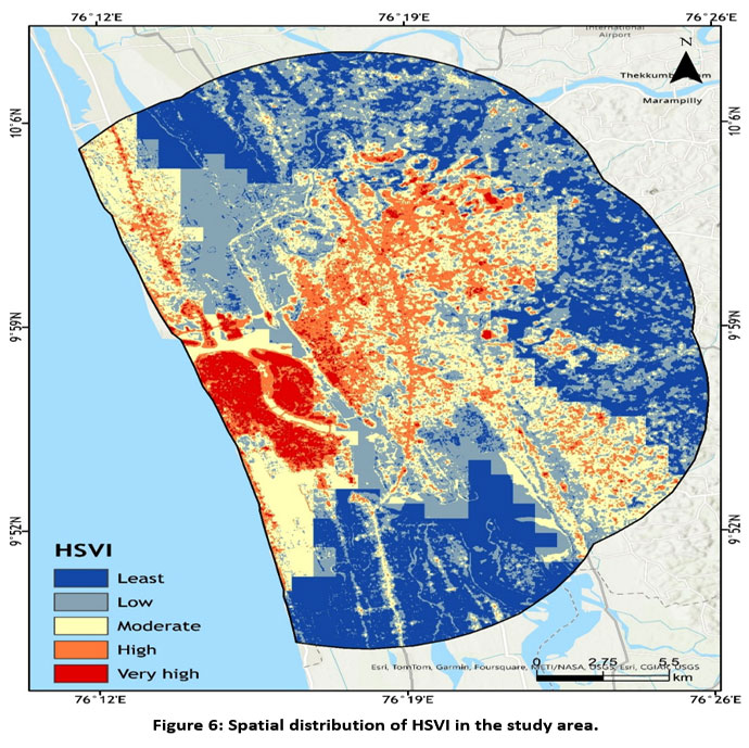 | Figure 6: Spatial distribution of HSVI in the study area.
|
The resultant HSVI is reclassified into five categories: very low, low, moderate, high, and very high vulnerability classes. Approximately 178 km2 (26.76%) of the study area is categorized as very low heat stress vulnerability, followed by 207 km2 (31.12%) in the low category, 172 km2 (25.86%) in moderate vulnerability, 85 km2 (12.78%) in high vulnerability, and 23 km2 (3.45%) in very high vulnerability. Higher HSVI is observed in the central region of the study area, while lower HSVI is observed towards the periphery. These high areas exhibit high built-up density and have undergone LULC changes over the study period.
The findings of this study align with previous research conducted under similar geo-environmental conditions. For instance, Mohammad and Goswami53 investigated LST variations and LULC changes in Ahmedabad city, India, and noted that intensive urban growth led to an increase in LST exceeding 45°C. Similarly, Tan54 studied LST over Penang Island, Malaysia, and found that areas with high urban density exhibited the highest LST among different LULC changes.
Discussion
Urbanisation, infrastructure development, and the migration of people are the main reasons for the changes in LU/LC. The unexpected rains, associated floods and other meteorological events also caused changes in LU/LC of the study area23. From 1988 to 2005, Kochi acted as the financial, industrial and commercial capital. The CSEZ and the Cochin Stock Exchange acted as the conduits for Kochi's investment prospects during this time.
The development of industrial infrastructures like the HMT, BPCL, FACT, and KINFRA accelerated the urbanisation in the study area.37 During this time, expeditious urbanisation took place in the central region of the city, which gradually moved to the periphery.38 In the subsequent years, the opening of Cochin International Airport and the development of its terminals added to the built-up area. Kochi has also seen fast urbanisation in the peripheries with the establishment of Smart city, Cochin Special Economic Zone, the Ship Repair centre and the LNG terminal (Puthuveypu). The establishment of the International Container terminal paved the way for an increase in transportation facilities like water metro, metro rail and a number of bridges, which added to the urbanisation. Some of the factors, like low-cost labour, good communication infrastructure and low real estate cost as compared to other metros in the country, have led to the urban development of Kochi in the past few years.39,40 Urbanization that takes place without proper planning and encroachment into ecologically vulnerable areas of Kochi have destroyed the city’s ability to cope with weather events. Since Kochi is a low-lying coastal city, these impacts are much aggravated.38
This conversion of vegetative cover into urbanized zones has led to a notable rise in temperature. The investigation reveals a direct correlation between LST and built-up areas, aligning with findings from a study conducted in urban regions of Italy by Morabito. 45 Impervious surfaces exert a considerable positive influence on LST. The percentage of imperviousness emerges as the most reliable predictor of LST, corroborating the outcomes of Zhou.44 These findings are consistent with earlier research by Yuan.45 Conversely, vegetation exhibits a substantial negative impact on LST, mirroring observations made in the colder Twin Cities Metropolitan Area of Minnesota,45 as well as the hotter and drier Phoenix metropolitan region of Arizona.46,47 In Kochi, the intensity of the Urban Heat Island was moderate to high in both the winter and summer, and it is thought to be positively correlated with urbanization.52 The correlation coefficient (r or R) serves as a measure of the degree of association between two variables - independent and dependent variables.50 The study concludes that spectral indices such as NDBI and NDVI are indeed linked to LST.40,41
Strong negative and positive correlations were observed between LST and NDVI for various LULC changes. Additionally, the present study highlights that urban area expansion contributes to increased LST, consistent with findings from Muhammad and Goswami53 in Ahmedabad city and Pradeep and Rupa Narayanan55 in Bilaspur district, Chhattisgarh, where increases in built-up area correlated with rising temperatures.
Moreover, urbanization, population growth, industrialization, and unsystematic land use planning can exacerbate heat stress vulnerability, particularly during extreme summer conditions.36 The present HSVI findings are in line with a study by Halder et al.,40 in Horan and Kolkata cities, India, where very high heat stress was linked to 17.35% of the area, primarily concentrated in the central, northern, and southeastern parts, attributed to high rates of building construction and densely built-up lands.
Conclusion
Land use and land cover (LULC) changes associated with an increase in land surface temperature (LST) pose a significant global concern. This study investigates the patterns of LULC change in Kochi city, India, utilizing multispectral, spatio-temporal data spanning 35 years from 1988 (Landsat 5 TM), 2005 (Landsat 7 ETM+), and 2023 (Landsat 8 OLI/TIRS). The study reveals a predominant conversion of land into built-up class, with a notable increase while categories such as vegetation and open areas exhibit a marked decline. Consequently, vegetation indices like NDVI indicate a loss of green cover, whereas the built-up index (NDBI) shows a gradual rise. These changes collectively contribute to an LST increase of 4.45°C from 1988 to 2023. The correlation of LST with NDVI and NDBI has shown R2 0.25 and 0.57, respectively. Temperature rises as built-up area grows due to the significant positive association between LST and NDBI. Healthy green vegetation decreases the surface temperature, as seen by the strong negative association between NDVI and LST. Therefore, it can be argued that NDBI offers a solid foundation for urban planning and construction, in addition to being able to assess and forecast LST and depict the urban heat island effect in any location.
Kochi city has been experiencing an Urban Heat Island (UHI) effect since 2000, coinciding with the surge in urban development. In response to these trends, the study proposes a Heat Stress Vulnerability Index (HSVI) using the Analytic Hierarchy Process (AHP). The HSVI delineates various vulnerability classes, as very low heat stress vulnerability,followed by low, moderate, high, and as very high vulnerability in the decreasing order of abundance.
Areas with higher HSVI are spatially concentrated in the central region of the study area. To mitigate the UHI effect and enhance sustainable development, the expansion of green spaces and creation of green buildings is deemed imperative and has significant contributions to the cooling effect of an area. Consequently, the study's findings serve as valuable insights for the future LST prediction so that policymakers, urban planners, in conjunction with public participation, can facilitate the formulation of mitigatory measures aimed at reducing LST and fostering greenery in tropical regions with high HSVI. These sustainable environmental conservation activities help to achieve Sustainable Development Goals 3 (SDG-3; good health and well-being) and 13 (climate action).
Acknowledgement
The author would like to thank the University of Kerala for granting the Ph.D. research work. The Department of Environmental Sciences, University of Kerala, is highly appreciated for allowing the GIS lab works. Also, profoundly grateful to the National Remote Sensing Center (NRSC), Indian Space Research Organisation (ISRO), Govt. of India, for their guidance during the Satellite data procurement.
Funding Sources
The authors received no financial support for the research, authorship, and/or publication of this article.
Conflict of Interest
The authors do not have any conflicts of interest.
Data Availability Statement
The manuscript incorporates all datasets produced or examined throughout this research study.
Ethics Statement
This research did not involve human participants, animal subjects, or any material that requires ethical approval.
Informed Consent Statement
This study did not involve human participants, and therefore, informed consent was not required.
Permission to reproduce material from other sources
Not Applicable
Author Contributions
Aswathy Asok: Methodology, writing, analysis editing
Sabu Joseph: Writing and editing, Supervision.
Asok Laila Achu: Methodology, writing and editing,
Girish Gopinath: Writing and resources,
Jobin Thomas: Methodology, writing and editing.
References
- Liu Z., Chunyang, H., Yuyu Z. and Jianguo W. How much of the world’s land has been urbanized. A hierarchical framework for avoiding confusion. Perspective. 2014; 29: 763–771.
CrossRef - Zhang Q. and Xing. The trends, promises and challenges of urbanisation in the world. Habitat International. 2016; 54: 241-252.
CrossRef - Winkler K., Fuchs R., Rounsevell M. and Herold M. Global land use changes are four times greater than previously estimated. Nat Comm. 20211; 2(1): 1–10.
- Ming L. and Lau N. C. Increasing heat stress in urban areas of eastern China: Acceleration by urbanization. Geophy Res Let, 2018; 45 (23): 1-21.
CrossRef - P. E. Kamil KMark MJay GBernadette PHumberto SRobert A. TUrban Heat Island: Mechanisms, Implications, and Possible Remedies. Ann Rev of Envt and Res, 2015; 40: 285-307.
CrossRef - Nayak S.G. , Shrestha S. , Kinney P.L., Ross Z. , Sheridan S.C. , Pantea C.I. , Hsu W.H. , Muscatiello N. and Hwang S.A. Development of a heat vulnerability index for New York State. Clinicalkey, 2018; 161: 127 – 137.
CrossRef - Thomas G., Sherin S., Ansar A.P. and Zachariah E.J. Analysis of Urban Heat Island in Kochi, India, Using a Modified Local Climate Zone Classification. Procedia Envt Sci. 2014; 21: 3-13.
CrossRef - Damla O. and Hatice D. Climate change and Food Security 2023; 1968-1979.
- Bendib A ., Hadda D. and Mohamed I. K. Contribution of Landsat 8 data for the estimation of land surface temperature in Batna city, Eastern Algeria. Geocarto International. 2017; 32:503 – 513.
CrossRef - Govind N. R. and Ramesh H. The impact of spatiotemporal patterns of land use land cover and land surface temperature on an urban cool island: a case study of Bengaluru. Environmental Monitoring and Assessment. 2019;191.
CrossRef - Oke T.R., Mills G., Christen A. and Voogt J.A. Urban Climate; Cambridge University Press: Cambridge. 2019: 64-76.
- Sultana S. and Satyanarayana A. N. V. Impact of urbanisation on urban heat island intensity during summer and winter over Indian metropolitan cities. Environ Monitor Assessment, 2019; 191(3): 789 - 806.
CrossRef - Ramamurthy A., Faiz A., Chundeli A., Chandran G. and Taruni J. Evaluating the Impact of Urbanisation on Climate Change: A Case of Kochi City, Kerala State, India. 2024.
- Singh R. and Grover A. Spatial correlations of changing land use, surface temperature (UHI) and NDVI in Delhi using Landsat satellite images. Urban Development Challenges, Risks and Resilience in Asian Mega Cities. 2014; 83-97.
CrossRef - Liu Q., Gu J., Yang J., Li Y., Sha D., Xu M. and Yang C. Cloud, edge, and mobile computing for smart cities. Urban Informatics. 2021; 757-795.
CrossRef - Dorghamy A. E. Heat Island effects and cities. Middle Eastern Cities in a Time of Climate Crisis. 2022; 231-234. https://doi.org/10.4000/books.cedej.8634.
CrossRef - Qu L., Wang Y., Shi C., Wang X., Masui N., Rötzer T. And Koike T. Vigor and health of urban green resources under elevated O3 in far East Asia. 2023.
CrossRef - Dhanya P. K. and Suresh S. Evaluation of Urban Land Surface Temperatures and Land Use/Land Cover Dynamics for Palakkad Municipality, Kerala, for Sustainable Management. Urban Commons, Future Smart Cities and Sustainability, 2023; 533-550.
CrossRef - Firoz M. C., Sruthi K. V. and Taniya V. Assessment of Land Surface Temperature Variations and Implications of Land Use/Land Cover Changes: A Case of Malappuram Urban Agglomeration Region, Kerala, India. International Journal of Built Environment and Sustainability, 2023; 10: 13-36.
CrossRef - World Population Prospects. Department of Economics and Social Affairs, Population Division, United Nations, New York. 2022.
- Kerala Sustainable Urban Development Project. Government of Kerala. 2005: 2.
- Thekkeyil A., Shijo J., Fathima A., Giby K., Nameer P. O. and Purushothaman C. A. Land use change in rapidly developing economies – A case study on land use intensification and land fallowing in Kerala, India. Research square. 2022;1-20.
CrossRef - Sánchez F. G. and Dhanapal G. 2023. Integrating blue-green infrastructure in urban planning for climate adaptation: Lessons from Chennai and Kochi, India. Land Use Policy, 124.
CrossRef - Vinod U. An Economic Evaluation of Special Economic Zones: A Study on Cochin Special Economic Zone in Kerala. 2017:15-18.
- Stewart I.D. and T. R. Oke. Local Climate Zones for Urban Temperature Studies. American Meteorological Society. 2012; 93:1879-1900.
CrossRef - Thomas G ., Jobin T., Mathew A. V., Devika R. S., Anju K. and Nair A. J. . Non-uniform effect of COVID-19 lockdown on the air quality in different local climate zones of the urban region of Kochi, India. Spatial Information Research. 2023; 31: 145-155.
CrossRef - Breiman L. Random Forests. 2001; 45: 5-32.
CrossRef - Breiman L. Bagging predictors. Machine Learning. 1996; 26(2): 123–140.
CrossRef - Breiman L., Jerome F., Olshen. R.A., Charles J. S. “Classification and regression trees”. 1984; 368.
- Gosh A., Sharma R. and Joshi P.K. Random Forest classification of urban landscape using Landsat archive and ancillary data: Combining seasonal maps with decision level fusion. Applied geography. 2014; 48:31-41.
CrossRef - Cohen. A coefficient for nominal scales. 1960; 20 (1): 37-46.
CrossRef - Carlson T. N. and Ripley D.A. On the relation between NDVI, fractional vegetation cover, and leaf area index. Remote Sensing of Environment. 62: 241-252.
CrossRef - Xu H. Extraction of Urban Built-up Land Features from Landsat Imagery Using a Thematic oriented Index Combination Technique. Photogrammetric Engineering & Remote Sensing. 2007; 73: 1382 – 1391.
CrossRef - Anupriya R. S. and Rubeena T. A. Spatio-temporal urban land surface temperature variations and heat stress vulnerability index in Thiruvananthapuram city of Kerala, India. Geology, Ecology and Landscapes. 2023; 9: 262-278.
CrossRef - Saaty T. The analytic hierarchy process (AHP) for decision making In Kobe, Japan. McGraw-Hill, New York, 1980: 1–69.
- Krishnaveni K.S. and Anil K. P. P. Spatio-temporal dynamics of urban sprawl in a rapidly urbanizing city using machine learning classification. Geocarto International. 2022; 37(27): 17403-17434.
CrossRef - George J. An Assessment of Inclusiveness in the Urban Agglomeration of Kochi City: The need for a change in the approach of urban planning. Munich Personal RePEc Archive (MPRA). 2016
- Kuriakose P. N. and Philip S. City profile: Kochi, city region-Planning measures to make Kochi smart and creative. 2021;118.
CrossRef - Halder B., Bandyopadhyay J., Al-Hilali A. A., Ahmed A. M., Falah M. W., Abed S. A., Falih K. T., Khedher K. M., Scholz M. and Yaseen Z. M. Assessment of urban green space dynamics influencing the surface urban heat stress using advanced geospatial techniques. Agronomy. 2022; 12.
CrossRef - Arulbalaji P., Padmalal D., and Maya K. Impact of urbanization and land surface temperature changes in a coastal town in Kerala, India. Environmental Earth Sciences. 2020; 79: 1–18.
CrossRef - Fensholt R., Tobias L., and Kjeld R. Greenness in semi-arid areas across the globe 1981–2007 - an Earth Observing Satellite based analysis of trends and drivers. Remote Sensing of Environment. 2012;121: 144–158.
CrossRef - Morabito M., Alfonso C., Alessandro M., Simone O., Antonio R., Giampie M. And Michele M.The impact of built-up surfaces on land surface temperatures in Italian urban areas. Science of the Total Environment, 551: 317-326.
CrossRef - Zhou W., Qian Y., Li X., Li W., and Han L.. “Relationships between land cover and the surface urban heat island: seasonal variability and effects of spatial and thematic resolution of land cover data on predicting land surface temperatures”. Landscape Ecology, 2013; 29(1): 153–167.
CrossRef - Yuan F. and Bauer M.E. Comparison of impervious surface area and normalized difference vegetation index as indicators of surface urban heat island effects in Landsat imagery. Remote Sensing of Environment. 2007; 106: 375–386.
CrossRef - Buyantuyev A. and Wu J. Urban heat islands and landscape heterogeneity: linking spatiotemporal variations in surface temperatures to land-cover and socioeconomic patterns. Landscape Ecology. 2010; 25(1): 17–33.
CrossRef - Jenerette G.D., Harlan S.L., Stefanov W.L. and Martin C.A. Ecosystem services and urban heat riskscape moderation: water, green spaces, and social inequality in Phoenix, USA. Ecological Application. 2011; 21: 2637–2651.
CrossRef - Mwangi P. W., Faith N. K. and Peter K. K. Analysis of the Relationship between Land Surface Temperature and Vegetation and Built-Up Indices in Upper-Hill, Nairobi. Journal of Geoscience and Environment Protection, 2018; 6.
CrossRef - Jalan S. and Sharma K. Spatio-temporal Assessment of Land Use/ Land Cover Dynamics and Urban Heat Island of Jaipur City using Satellite Data”. ISPRS. 2014; XL.
CrossRef - Senthilnathan S. Usefulness of Correlation Analysis. SSRN. 2019; 9.
CrossRef - Kim S. W. and Brown R. D. Urban heat island (UHI) variations within a city boundary: A systematic literature review. Renewable and Sustainable Energy Reviews. 2019;148.
CrossRef - Thomas G. and Zachariah E.J. Urban Heat Island in a Tropical City Interlaced by Wetlands”. Journal of Environmental Science and Engineering. 2011; 5.
- Muhammad P., and Ajanta G. The Impact of the Land Cover Dynamics on Surface Urban Heat Island Variations in Semi-Arid Cities: A Case Study in Ahmedabad City, India, Using Multi-Sensor/Source Data. Remote sensing of climate change. 2022; 19.
CrossRef - Tan K.C., Lim H.S., Mat M.Z., Jafri K., Abdullah. Study on Land Surface Temperature Based on Landsat Image over Penang Island, Malaysia. Sixth International Conference on Computer Graphics, Imaging and Visualization. 2009.
CrossRef - Pradeep V., and Rupanarayanan. “Estimation of Land Surface Temperature in selected Tehsil of Bilaspur district in Chhattisgarh, India using GIS & Remote Sensing Technique”. IJARIIE. 2020; 6.
- Lowry, W. P. The Climate of Cities. Scientific American, (1967). 217(2), 15–23. http://www.jstor.org/stable/24926081
CrossRef