Current World Environment

Introduction

Rainfall is important yet difficult weather variables to predict, influencing agriculture, flood risk, and water availability. Accurate daily rainfall forecasting is therefore crucial for agricultural planning, irrigation management, food security, and flood disaster prevention.^1–3 Even after many years of progress in atmospheric science, predicting daily rainfall is still very difficult, especially in monsoon regions where rainfall is heavy, unevenly distributed, and influenced by complex atmospheric processes.^4,5 One region where this challenge is particularly relevant is Assam in northeast India. The state is among the most flood-prone regions in the world, with nearly 40% of its land area at risk, compared to a national average of around 12%. ⁶ The 2022 Assam floods caused extensive agricultural devastation, inundating over 2.45 million hectares of land across multiple districts and severely impacting rice production, as quantified through satellite-based monitoring.⁷ For rice-growing communities in Assam, even a small improvement in one-day rainfall forecasts can help farmers decide the right time for sowing and reduce the risk of crop loss. However, reliable and region-specific daily rainfall prediction tools for Assam are still limited.

Over the years, machine learning has emerged as a powerful and flexible alternative to both traditional statistical approaches and computationally expensive numerical weather prediction (NWP) models for precipitation forecasting.^3,8 Multiple Linear Regression (MLR) has long been used as a basic method because it is simple and easy to interpret. However, rainfall processes are highly nonlinear and complex, and linear models often fail to capture these patterns. As a result, many studies have shown that machine learning methods usually perform better than traditional regression models in predicting rainfall under complex meteorological conditions.^9,10

Extreme Gradient Boosting (XGBoost¹¹ has become one of the most widely applied algorithms for meteorological prediction. Across South Asia, benchmarking studies have confirmed that XGBoost consistently outperforms classical statistical approaches including ARIMA and regression in capturing the nonlinear dynamics of monsoon precipitation.^12,13 Hybrid frameworks combining XGBoost with deep learning have achieved remarkable accuracy in Bangladesh, with RMSE as low as 0.65 mm/day,¹⁴ while studies across northern India have similarly found gradient boosting approaches to outperform linear and regularisation-based methods for daily rainfall forecasting.^9,10 XGBoost has also been successfully applied to bias-correct NWP precipitation output across climatically diverse regions of China, substantially improving short-term forecast skill.¹⁵ Light Gradient Boosting Machine (LightGBM) has gained increasing attention for its computational efficiency and strong predictive performance. In urban rainfall–runoff prediction, it has outperformed LSTM networks while requiring significantly lower computational cost.¹⁶ For extreme precipitation prediction, ensemble models combining LightGBM with CatBoost have consistently outperformed linear approaches,¹⁷ and LightGBM has demonstrated strong skill in probabilistic spatial prediction of precipitation, particularly at extreme quantiles.¹⁸ Comprehensive assessments of Indian climate trends using both XGBoost and LightGBM have confirmed that these models enhance rainfall forecasting accuracy and provide actionable insights for agricultural and disaster management planning.^19,20

Despite this growing literature, several important gaps remain. Most machine learning rainfall studies in India focus on large spatial scales, whereas region-specific analyses required for flood and agricultural management, particularly in Northeast India, remain limited.^8,21 Second, the vast majority of studies evaluate models using only continuous metrics such as RMSE and R², without reporting categorical event-detection performance across multiple intensity thresholds, information that is indispensable for flood early warning and crop scheduling applications.^1,2 Third, few studies implement strict temporal train-test separation, raising the risk of data leakage inflating reported performance figures.⁹ Finally, systematic seasonal evaluation of model skill across multiple hydro-climatic regions is rarely reported.^15,22

To address these gaps, this study develops and evaluates Multiple Linear Regression, XGBoost, and LightGBM for daily rainfall prediction across five hydro-climatic regions of Assam: Barak Valley, Central Assam, Lower Assam, Upper Assam, and North Assam using a 24-year dataset (2001–2024) and a strict temporal validation protocol. The specific objectives are to: (i) compare continuous prediction accuracy across all three models and five regions; (ii) evaluate categorical event-detection skill at different rainfall intensity thresholds; (iii) decompose seasonal model performance.

Materials and Methods

This study employs a multi-model framework to forecast daily precipitation across five agro-climatically distinct regions of Assam — Barak Valley, Central Assam, Lower Assam, Upper Assam, and North Assam. Three machine learning and statistical models were developed and compared: Multiple Linear Regression (MR), Extreme Gradient Boosting (XGBoost), and Light Gradient Boosting Machine (LightGBM). The methodology encompasses five interconnected phases: (i) study area delineation and station coverage, (ii) data acquisition and preprocessing, (iii) feature engineering, (iv) model development and temporal validation, and (v) performance evaluation.

Study Area and Data

This study focuses on rainfall forecasting across five hydro-climatically distinct sub-regions of Assam, India: Barak Valley, Central Assam, Lower Assam, Upper Assam, and North Assam (Figure 1). These regions represent different physiographic and climatic regimes within the Brahmaputra–Barak river basin system, including lowland floodplains, foothill zones, and areas influenced by complex orographic effects. For each hydro-climatically distinct region of Assam, a representative grid point was selected to extract daily rainfall and meteorological variables. The geographic coordinates and elevation of these representative data points are summarized in Table 1.

Table 1: Representative meteorological data points used for each hydro-climatic region of Assam.

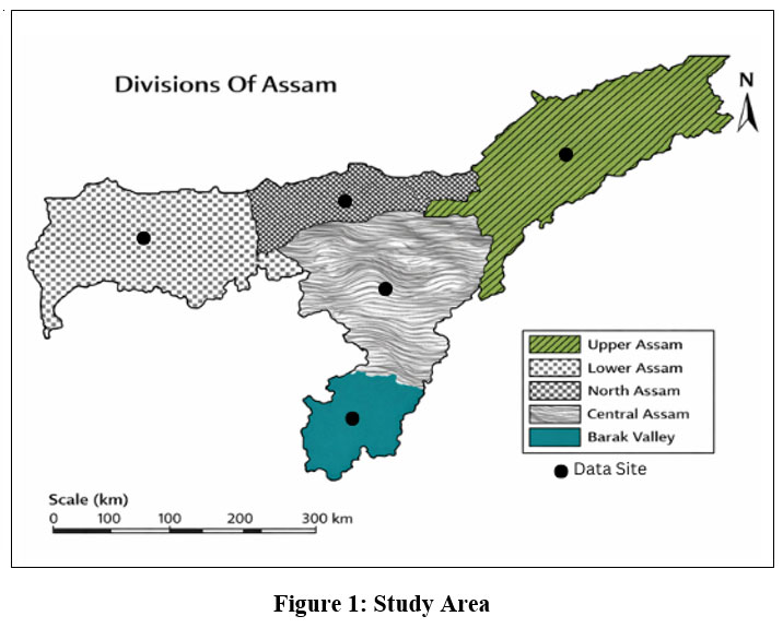Figure 1: Study Area Click here to view Figure

Daily meteorological observations were collected for representative stations located within each region. The dataset spans January 2001 to December 2024, providing a continuous 24-year record of rainfall and associated atmospheric variables. Table 2 presents the variables used in this study along with their respective sources.

Table 2: Meteorological Variables Used in the Study

Daily meteorological data for each region were obtained and stored in Microsoft Excel (.xlsx) format. Before modelling, the data were carefully pre-processed to ensure consistency and to avoid any leakage of information between the training and testing periods. Column names were cleaned by removing extra spaces, and checks were performed to ensure that all variables were present. The dataset was examined for missing values, and none were found in the collected data. During feature engineering, the first few rows were automatically removed because lag variables create undefined values at the beginning of the time series. For the Multiple Regression model, all predictor variables were standardised using z-score scaling, where the scaling parameters were calculated only from the training data. In contrast, the tree-based models (XGBoost and LightGBM) were used without scaling since they are not sensitive to the magnitude of input variables. Finally, because precipitation cannot be negative, any negative predictions produced by the regression model were set to zero before calculating the evaluation metrics.

Feature Engineering

Several additional features were created to improve the predictive performance of the machine learning models which represented seasonal behaviour and short-term temporal relationships in rainfall. These engineered features were used only for the XGBoost and LightGBM models, while the Multiple Regression model used only the original meteorological variables. The base variables included All Sky Surface Shortwave Downward Irradiance, Dew/Frost Point, Maximum and Minimum Temperature, Specific Humidity, Surface Pressure, Wind Speed, Surface Soil Wetness, and Precipitation.

First, a month variable was extracted from the date column to represent the seasonal cycle of rainfall. Because rainfall in Assam follows a strong monsoon-driven seasonal pattern, this variable helps the model recognise differences between months such as pre-monsoon, monsoon, and post-monsoon periods. To avoid the artificial gap between December and January, the month variable was converted into two cyclic variables using sine and cosine transformations.

These two variables allow the model to represent the annual cycle smoothly.

Next, lag features were created for each meteorological variable to represent conditions from previous days. Specifically, three lag variables were generated: the value of the variable on the previous day, two days earlier , and three days earlier. For example, the lag feature temperature_lag_1 represents the temperature recorded one day before the current prediction day. These lag variables were generated using a simple time-shift operation on the dataset. Including these variables allows the models to learn how recent weather conditions influence rainfall on the current day.

Moreover, rolling statistics were also created to capture short-term trends in atmospheric conditions. For each meteorological variable, a three-day rolling mean was calculated using the current day and the two preceding days. This rolling average smooths short-term fluctuations and captures the recent overall atmospheric conditions. For example, the rolling mean of temperature represents the average temperature over the last three days.

These engineered variables were then included as input features for the XGBoost and LightGBM models, allowing them to capture both seasonal patterns and short-term persistence in meteorological conditions. However, the Multiple Regression model did not use these engineered features, because including many correlated lag variables could introduce multicollinearity and reduce the stability of the regression coefficients.

Model Development and Temporal Validation

Temporal Train/Test Split Strategy

Special care was taken to prevent any information from the test period from influencing model training. The dataset was first arranged in strict chronological order so that all lag and rolling features were created using only past observations.²³ The data were then divided based on time, with records from 2001–2023 used for model training and the independent year 2024 reserved for testing. Hyperparameter optimization was carried out exclusively on the training data using GridSearchCV with three-fold cross-validation. The dataset was partitioned into three equal segments, where in each iteration two segments were utilized for training and the remaining segment for validation.²⁴ This process was repeated three times, allowing each segment to function as the validation set once. The optimal hyperparameters were then determined based on the average validation error across all folds. This approach helps reduce overfitting and improves model generalisation. For the Multiple Regression model, predictor variables were standardised using parameters calculated only from the training data, which were then applied to the test data without recalculation. Because lag and rolling features were generated using only previous time steps, no future information was included.²³ These steps ensured that the modelling process remained realistic and free from information leakage.

Multiple Regression Model

Multiple Linear Regression was used as a statistical baseline model. The relationship between rainfall and meteorological predictors is expressed as:

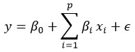
Where y represents daily rainfall, x_i are predictor variables, B_i are regression coefficients, and E represents model error. The regression coefficients were estimated using ordinary least squares after standardizing predictor variables.

XGBoost Model

Rainfall forecasting was performed using Extreme Gradient Boosting (XGBoost) regression, an ensemble learning technique that constructs an additive model of decision trees optimized via gradient descent.^13,25

Let {(x_i, y_i)}^N_i=1 denote the training dataset, where x_i is the feature vector and y_i is the observed rainfall. The predicted rainfall y_i is given by:

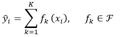
where each f_k represents a regression tree and F denotes the space of all possible trees. The objective function minimized by XGBoost is:

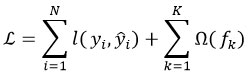
where l(.) is the loss function and n(f_k) is a regularization term controlling model complexity.

For this study, the squared error loss was adopted:

and the regularization term is defined as:

where T is the number of leaves in a tree, w_j represents the leaf weights, and Y and h are regularization parameters penalizing model complexity.²⁶ This formulation enables XGBoost to control overfitting while efficiently capturing nonlinear interactions among meteorological variables.^14,15

LightGBM

In addition to XGBoost, rainfall forecasting was also performed using the Light Gradient Boosting Machine (LightGBM) algorithm. LightGBM is a gradient boosting framework developed by Microsoft that builds an ensemble of decision trees in a sequential manner to minimize prediction error. Similar to XGBoost, LightGBM optimizes an objective function consisting of a loss function and a regularization term, allowing the model to learn complex nonlinear relationships between predictor variables and the target variable.²⁷

LightGBM incorporates several methodological enhancements that improve its computational efficiency, particularly when handling large datasets. To begin with, it adopts a leaf-wise tree growth strategy, in which the leaf contributing the highest reduction in loss is split, rather than expanding the tree level by level. This enables the model to attain higher predictive performance with fewer boosting iterations. Additionally, LightGBM utilizes a histogram-based approach for decision tree construction, where continuous features are discretized into bins, leading to substantial reductions in both memory consumption and training time. Furthermore, it integrates Gradient-based One-Side Sampling (GOSS), which focuses on instances with larger gradient values, and Exclusive Feature Bundling (EFB), which combines mutually exclusive sparse features to effectively reduce dimensionality.²⁸

These characteristics enable LightGBM to efficiently model complex nonlinear relationships in meteorological data while maintaining high computational efficiency. In this study, the LightGBM model was trained using the same predictor variables and evaluation framework as the XGBoost model to allow a fair comparison of rainfall prediction performance.

Hyperparameter Optimisation

For both XGBoost and LightGBM, optimal hyperparameters were identified through exhaustive grid search cross-validation (GridSearchCV, sklearn) with 3-fold cross-validation on the training partition, using negative mean squared error as the scoring criterion.In 3-fold cross-validation, the training data were split into three subsets, with two folds used for training and one for validation in each iteration, and the average validation error across folds was used for hyperparameter selection.²⁹ The hyperparameter grids are summarised below.

XGBoost search grid: learning_rate E {0.1, 0.2, 0.5, 1}, max_depth E {3, 5, 8}, n_estimators E {50, 100, 200}, subsample = {1.0}. The objective function was set to reg:squarederror, and random_state = 42 was fixed throughout.

LightGBM search grid: learning_rate E {0.05, 0.1, 0.2, 0.5}, max_depth E {3, 5, 8}, n_estimators E {50, 100, 200}, num_leaves E {31, 63}, subsample E {0.8, 1.0}. The objective was set to regression and random_state = 42 was fixed throughout. The wider num_leaves parameter specifically leverages LightGBM's leaf-wise tree growth, which can achieve lower bias than the level-wise strategy used by XGBoost for equivalent tree depth.

Seasonal Decomposition of Results

Beyond overall annual performance on the 2024 test year, results were disaggregated into four meteorological seasons relevant to the northeast Indian climate: Winter (December–February; DJF), Pre-Monsoon (March–May; MAM), Monsoon (June–September; JJAS), and Post-Monsoon (October–November; ON). This seasonal stratification allows examination of model skill across low-precipitation and high-precipitation regimes and reveals whether model accuracy degrades during the climatologically challenging peak monsoon period.

Model Evaluation and Skill Metrics

Model performance was evaluated using both continuous and categorical metrics, ensuring alignment with the Results section.

Continuous Metrics

Coefficient of Determination (R²): R-squared, also known as the coefficient of determination, is used to measure the proportion of the variance in the dependent variable that can be predicted from the independent variables.³⁰ It is defined as

Mean Absolute Error (MAE): It represents the average absolute difference between predicted and actual values, offering a clear measure of typical prediction error in the same units. It is given by:

Root Mean Squared Error (RMSE): It calculates the square root of the mean squared deviations between predictions and observations, placing greater emphasis on larger errors and indicating model accuracy. It is given by

Event-based Metrics

Daily precipitation data usually contain many zero-rainfall days, and important rainfall events occur at different intensity levels. Therefore, relying only on continuous evaluation metrics is not sufficient to assess the performance of rainfall prediction models. To better evaluate the ability of models to detect rainfall events, categorical metrics—Probability of Detection (POD), False Alarm Ratio (FAR), and Critical Success Index (CSI)—were calculated.

These metrics were evaluated at seven rainfall thresholds: 0.1, 0.5, 1.0, 2.5, 5.0, 10.0, and 25.0 mm/day. These thresholds were selected to represent progressively increasing rainfall intensities—from very light precipitation to heavy rainfall events, allowing evaluation of model performance across different meteorological and hydrological impact levels. For each threshold, observed and predicted rainfall values were converted into binary events, where rainfall exceeding the threshold was considered an event, and otherwise a non-event. Using the resulting contingency table counts (True Positives, False Positives, and False Negatives), POD, FAR, and CSI were calculated separately for each region and model.

Probability of Detection (POD): It assesses the model’s sensitivity to rainfall events by measuring its ability to capture observed occurrences. We write

False Alarm Ratio (FAR): It is crucial for evaluating the reliability of the model and defined as

Critical Success Index (CSI): It is used to evaluate the accuracy of rainfall forecasts, it is defined as

The complete methodological workflow adopted in this study is summarised in Figure 2.

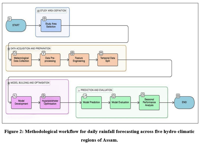Figure 2: Methodological workflow for daily rainfall forecasting across five hydro-climatic regions of Assam. Click here to view Figure

Results

This section presents the performance of the Multiple Regression (MR), XGBoost, and LightGBM, evaluated on the test year 2024 across five hydro-climatic regions of Assam. Results are reported using continuous metrics (R², MAE, RMSE), categorical detection metrics at multiple rainfall thresholds (CSI, POD, FAR), and seasonal decomposition of model accuracy.

Overall Continuous Performance

Table 3 summarises overall performance of all three models across the five regions. The gradient boosting models substantially outperformed Multiple Regression across every region and every metric, which clearly shows that the nonlinear relationships between meteorological variables and daily rainfall cannot be adequately captured by a linear framework.

Table 3: Comparative performance of Multiple Regression, XGBoost, and LightGBM models for daily rainfall prediction across the hydro-climatic regions of Assam (2024 test year).

Multiple Regression produced weak R² values ranging from 0.41 (Lower Assam) to 0.51 (Barak Valley), with high errors that reflect its inability to model the sharp intensity peaks typical of monsoon rainfall. In contrast, XGBoost and LightGBM achieved R² values between 0.78 and 0.97, reducing MAE by 60–85% and RMSE by 30–78% compared to the linear baseline, depending on region.

Lower Assam stood out as the region where both gradient boosting models performed best, with XGBoost reaching R² = 0.973, MAE = 0.791 mm, and RMSE = 1.943 mm, while LightGBM achieved near-identical scores (R² = 0.974). Central Assam also showed strong performance, with both models attaining R² above 0.93 and MAE well below 1 mm. Upper Assam proved most challenging: XGBoost achieved R² = 0.853 while LightGBM reached only 0.775, with LightGBM showing considerably higher RMSE (7.129 mm vs. 5.757 mm), suggesting that LightGBM's leaf-wise growth strategy may overfit to training patterns in this orographically complex region.

The temporal agreement between observed and predicted rainfall is illustrated visually in Figure 3 for XGBoost in Barak Valley, representing the overall model behaviour across the 2024 test year. Equivalent time-series plots for LightGBM and all remaining regions are provided in Appendix B (Figures B1–B9).

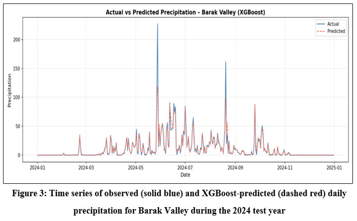Figure 3: Time series of observed (solid blue) and XGBoost-predicted (dashed red) daily precipitation for Barak Valley during the 2024 test year Click here to view Figure

Categorical Detection Performance

To assess how well the models can identify the occurrence of rainfall events at practically meaningful intensity levels, categorical metrics: CSI, POD and FAR were calculated at seven thresholds: 0.1, 0.5, 1.0, 2.5, 5.0, 10.0, and 25.0 mm/day. Table 4 presents the results at the 5.0 mm/day threshold, which represents a meteorologically relevant boundary between light and moderate rainfall and is commonly used in operational hydro-meteorological applications. Results at all remaining thresholds are provided in Appendix A (Tables A1–A6).

Table 4: Categorical detection performance of rainfall prediction models at the 5.0 mm/day threshold across the hydro-climatic regions of Assam (2024 test year).

Note. Higher CSI and POD, and lower FAR, indicate better event detection skill.

Across all regions and thresholds, XGBoost and LightGBM substantially outperformed Multiple Regression in categorical detection skill. At the 5 mm/day threshold, gradient boosting CSI values ranged from 0.852 to 0.958 compared to 0.533–0.631 for MR — a gain of roughly 0.30 to 0.40 CSI units. POD for both gradient boosting models consistently exceeded 0.93, meaning the models correctly identified more than 93% of rainfall events meeting or exceeding 5 mm/day. FAR was kept very low, particularly for XGBoost in Central Assam (FAR = 0.017) and North Assam (FAR = 0.022), demonstrating minimal false alarms.

As the rainfall threshold increased, all models experienced a decline in POD and CSI. However, the gradient boosting models maintained strong detection capability even at the most demanding threshold of 25 mm/day, with CSI values reaching as high as 0.964 (LightGBM, Upper Assam) and 0.943 (LightGBM, Barak Valley). Multiple Regression, by contrast, collapsed at this threshold, with CSI near zero in some regions. The threshold-dependent behaviour of CSI, POD, and FAR is visualised in Figure 4 for XGBoost in Barak Valley. Equivalent event-metric profiles for LightGBM and all other regions are shown in Appendix C (Figures C1–C9).

Figure 4: Event-based detection metrics for XGBoost in Barak Valley. Click here to view Figure

Seasonal Performance

Table 5 presents the seasonal R² values for XGBoost and LightGBM disaggregated into four meteorological seasons.

Table 5: Seasonal performance of XGBoost and LightGBM rainfall prediction models across hydro-climatic regions of Assam (2024 test year).

Note. R² values are computed separately for each season over the 2024 test year. Seasonal decomposition was not computed for Multiple Regression due to its markedly inferior overall performance.

Both models demonstrated exceptionally high skill during Winter and Post-Monsoon seasons, with R² consistently above 0.90 across all regions. Pre-Monsoon performance was also strong in most regions, with XGBoost reaching R² = 0.985 in both Central Assam and Upper Assam. The main exception was Barak Valley (XGBoost R² = 0.821; LightGBM R² = 0.796), reflecting the more erratic convective onset in this southernmost region.

The Monsoon season (June–September) produced the greatest spread in model performance, which is expected given that this period accounts for 70–80% of annual rainfall and is characterised by high temporal variability, intense convective events, and complex orographic interactions. Central Assam, Lower Assam, and Barak Valley maintained high monsoon R² values (0.889–0.959). However, Upper Assam showed a notable drop in skill, with XGBoost reaching R² = 0.796 and LightGBM only 0.687, consistent with the highly localised nature of orographic monsoon rainfall in the eastern Brahmaputra basin. Season-wise time series of observed versus predicted precipitation for all regions and models are shown in Figure 5 (Barak Valley, XGBoost) and in Appendix D (Figures D1–D9).

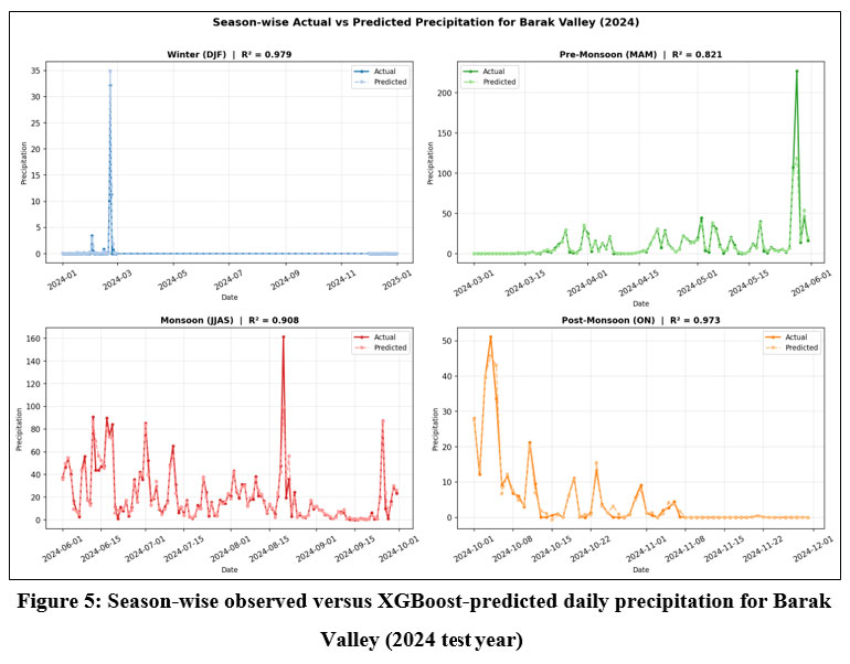Figure 5: Season-wise observed versus XGBoost-predicted daily precipitation for Barak Valley (2024 test year). Click here to view Figure

Discussion

This study demonstrates that gradient boosting machine learning models, particularly XGBoost and LightGBM, provide a strong and promising baseline framework for daily rainfall forecasting across the hydro-climatically diverse sub-regions of Assam. The findings are discussed here in the context of model capability, regional geography, the role of feature engineering, and the practical implications for agro-hydrological decision making.

Superiority of Gradient Boosting Over Linear Regression

The clear improvement of gradient boosting models over Multiple Regression confirms an important principle in rainfall modelling: the relationship between atmospheric variables and daily rainfall is highly nonlinear. In monsoon-dominated regions like Assam, rainfall is influenced by complex processes such as moisture convergence, convective activity, and orographic uplift. These interactions are difficult to represent using simple linear relationships. As a result, XGBoost and LightGBM achieved much higher accuracy (R² = 0.775-0.974; MAE = 0.738-1.902 mm) compared to Multiple Regression, which produced much lower R² values (0.41-0.51). Similar improvements of machine learning models over linear regression have also been reported in other rainfall studies across South and Southeast Asia.

The diagnostic plots for Multiple Regression (Figure 6) further highlight the model’s limitations. The observed-versus-predicted scatter, residual plots, and error distributions show that prediction errors increase as rainfall intensity increases. This fan-shaped pattern is typical when linear models are applied to highly skewed data such as daily rainfall. The residual distribution is also right-skewed, indicating that the model tends to underestimate heavy rainfall events. The event-based metrics provide similar evidence: the Probability of Detection (POD) decreases sharply above the 5 mm/day threshold, showing that the model struggles to detect stronger rainfall events. Diagnostic plots for the other regions are provided in Appendix E (Figures E1-E4).

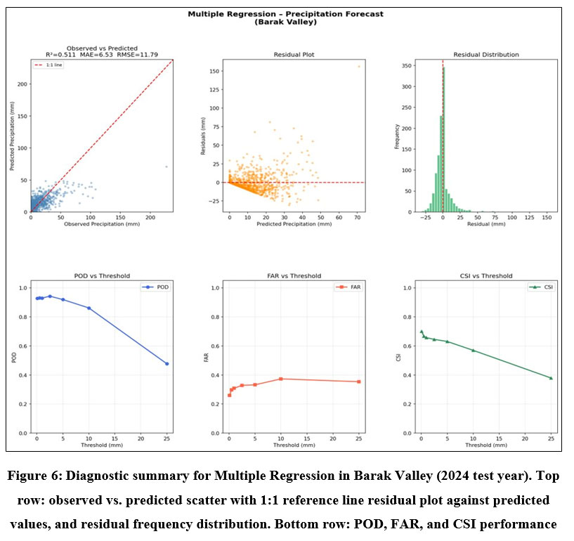Figure 6: Diagnostic summary for Multiple Regression in Barak Valley (2024 test year). Top row: observed vs. predicted scatter with 1:1 reference line residual plot against predicted values, and residual frequency distribution. Bottom row: POD, FAR, and CSI performance. Click here to view Figure

The collapse of Multiple Regression at the 25 mm/day categorical threshold, reaching CSI = 0 in Central Assam is particularly revealing. Linear models cannot extrapolate into the upper tail of the rainfall distribution because they are structurally constrained to produce outputs bounded by the training data's linear response surface. Gradient boosting trees, by contrast, can partition the input feature space and assign different response functions to high-intensity meteorological states, which is precisely what is needed for extreme event detection.

Regional Differences in Model Performance

The noticeable performance difference between Lower Assam (R² up to 0.974) and Upper Assam (R² as low as 0.775 for LightGBM) highlights the influence of regional geography on rainfall prediction. Lower Assam lies in the wide Brahmaputra floodplain, where rainfall is mainly controlled by large-scale weather systems. This makes rainfall patterns more predictable using grid-based meteorological variables. In contrast, Upper Assam is located near the foothills of the eastern Himalayas, where rainfall is strongly influenced by local terrain and orographic effects. These processes create highly variable rainfall patterns that are difficult to capture using single grid-point predictors.

The relatively weaker monsoon performance of LightGBM in Upper Assam (R² = 0.687 compared to XGBoost R² = 0.796) may be related to the model’s leaf-wise tree growth strategy, which can sometimes overfit complex or irregular patterns. The hyperparameter search used in this study may also not have fully explored the optimal settings for such a complex region. Future studies could improve performance by applying region-specific hyperparameter tuning methods, such as Bayesian optimisation, especially for areas with strong terrain influences.

Barak Valley showed strong overall model performance, but slightly lower R² values during the pre-monsoon season (XGBoost 0.821; LightGBM 0.796). This period is dominated by convective storms that occur more randomly and are less directly related to the large-scale atmospheric variables used as predictors. Because of this inherent randomness, predicting pre-monsoon rainfall remains challenging for both machine learning and traditional forecasting methods.

Value of Feature Engineering

The inclusion of lag features (t-1, t-2, t-3 days) and three-day rolling means for all meteorological variables gave the gradient boosting models memory of recent atmospheric states, a critical property for precipitation prediction. Rainfall in Assam, especially during the monsoon, exhibits strong temporal autocorrelation: once a large-scale moisture event is established, it tends to persist over multiple days. The cyclic encoding of month was equally important, allowing the models to learn the sharp seasonal transition between the dry winter and the intense monsoon without introducing an artificial discontinuity at the December-January boundary.

Practical Implications for Assam's Agro-Hydrological Sector

Assam faces recurring consequences from both rainfall deficit and excess. Kharif rice is deeply sensitive to rainfall timing and intensity during the June–September monsoon. Flood-prone districts in the Brahmaputra valley experience inundation cycles that damage crops, displace populations, and strain disaster response systems. A CSI of 0.958 at the 5 mm/day threshold (XGBoost, Central Assam) means that nearly 96% of rainfall events of agronomic or hydrological significance are correctly classified. A FAR of 0.022 (XGBoost, North Assam at the 5 mm/day threshold) indicates a very low false-alarm rate, meaning that only about 2.2% of predicted rainfall events were not actually observed.

The weakest performance was observed in Upper Assam, which is precisely the sub-region most vulnerable to flash flooding from rapid orographic enhancement of monsoon rain. This limitation should be communicated clearly to potential end users, and the development of ensemble or multi-model approaches is strongly recommended for this region.

Limitations and Future Directions

Several limitations deserve acknowledgement. First, all models are trained on data from a single representative grid point per region, which necessarily smooths over sub-regional heterogeneity. Second, the models use same-day meteorological predictors drawn from the NASA POWER reanalysis, which act as effectively perfect predictors. In a true operational setting, predictors would need to come from a numerical weather prediction (NWP) forecast for the lead time of interest, and evaluating model performance when driven by NWP ensemble output is an important next step. Third, climate non-stationarity — particularly the observed intensification of extreme rainfall events in northeast India under ongoing climate change — means that models trained on historical data may underperform as precipitation regimes shift.

Future work should explore atmospheric circulation indices, convective instability parameters, and satellite-derived moisture fields as additional predictors. Deep learning architectures may also be worth evaluating, particularly for capturing multi-day persistence structures across stations simultaneously.

Conclusion

This study evaluated three data-driven models: Multiple Regression, XGBoost, and LightGBM for daily rainfall prediction across five agro-climatically distinct regions of Assam, India, using a strict temporal validation protocol on the 2024 test year. Gradient boosting models dramatically outperformed Multiple Regression across all regions, all continuous metrics, and all categorical detection thresholds. The superiority of nonlinear tree-based models over linear regression is not merely incremental; it is fundamental, and should be considered a baseline expectation in any future work on daily rainfall forecasting in monsoon-dominated climates.

XGBoost and LightGBM delivered high prediction accuracy (R² = 0.775-0.974), with the best performance in Lower Assam and Central Assam and the most challenging conditions in Upper Assam. The performance difference between the two gradient boosting models was generally small but consistent, with XGBoost showing a slight edge in orographically complex and variable regions. At the event-detection level, both models achieved CSI values above 0.85 across most regions and thresholds, with POD consistently exceeding 0.93 and FAR below 0.10 at the 5 mm/day threshold. Even at the extreme 25 mm/day threshold, the gradient boosting models maintained practical detection skill entirely beyond the reach of linear regression.

Seasonal analysis showed that model performance was highest during Winter and Post-Monsoon, while skill was more variable during the Monsoon. The largest reduction in accuracy occurred in Upper Assam, where complex terrain and orographic rainfall processes make prediction more difficult using large-scale grid-point variables. These results suggest that machine learning models can provide useful support for rainfall forecasting in Assam, particularly for agriculture and flood risk management. However, further improvements are needed, especially in regions and seasons with highly variable rainfall. Future work should consider integrating these models with numerical weather prediction (NWP) forecasts, higher-resolution observational data, and uncertainty estimation methods to improve their reliability for operational forecasting in northeast India.

Acknowledgement

The authors gratefully acknowledge the India Meteorological Department (IMD) for providing the long-term monthly rainfall and temperature data used in this study.

Funding Sources

The authors received no financial support for the research, authorship, and/or publication of this article.

Conflict of Interest

The authors declare no conflict of interest.

Data Availability Statement

The manuscript incorporates all datasets produced or examined throughout this research study. Rainfall and temperature data used in this study were obtained from the India Meteorological Department (IMD). Other Satellite-derived meteorological variables were retrieved from the NASA POWER database.

Ethics Statement

This research did not involve human participants, animal subjects, or any material that requires ethical approval.

Informed Consent Statement

This study did not involve human participants, and therefore, informed consent was not required.

Permission to reproduce material from other sources

Not Applicable

Author Contributions

Nitesh Bothra: Data Collection, Analysis, Visualisation, Writing – Original Draft.

Surobhi Deka: Conceptualisation, Methodology, Writing – Review & Editing and Supervision.

References

1. Neyestani A, Asgari F, Asgari V. Application of Machine and Deep Learning Models to Forecast Daily Precipitation Over the Western Part of Iran. Meteorological Applications. 2025;32(6). doi:10.1002/met.70143
   CrossRef
2. Mohammed MH, Latif SD. Forecasting daily rainfall in a humid subtropical area: an innovative machine learning approach. Journal of Hydroinformatics. 2024;26(7):1661-1672. doi:10.2166/hydro.2024.016
   CrossRef
3. Liyew CM, Melese HA. Machine learning techniques to predict daily rainfall amount. J Big Data. 2021;8(1):153. doi:10.1186/s40537-021-00545-4
   CrossRef
4. Salaeh N, Ditthakit P, Pinthong S, Hasan MA, Islam S, Mohammadi B, et al. Long-Short Term Memory Technique for Monthly Rainfall Prediction in Thale Sap Songkhla River Basin, Thailand. Symmetry (Basel). 2022;14(8):1599. doi:10.3390/sym14081599
   CrossRef
5. Sharma D, Das S, Chakraborty D, Mitra A, Goswami BN. Improving Indian summer monsoon rainfall prediction using deep learning up to two years in advance. Quarterly Journal of the Royal Meteorological Society. 2026;152(774). doi:10.1002/qj.70023
   CrossRef
6. Borah L, Kalita B, Boro P, Kulnu AS, Hazarika N. Climate change impacts on socio-hydrological spaces of the Brahmaputra floodplain in Assam, Northeast India: A review. Frontiers in Water. 2022;4. doi:10.3389/frwa.2022.913840
   CrossRef
7. Halder B, Barman S, Banik P, Das P, Bandyopadhyay J, Tangang F, et al. Large-Scale Flood Hazard Monitoring and Impact Assessment on Landscape: Representative Case Study in India. Sustainability. 2023;15(14):11413. doi:10.3390/su151411413
   CrossRef
8. Wani OA, Mahdi SS, Yeasin Md, Kumar SS, Gagnon AS, Danish F, et al. Predicting rainfall using machine learning, deep learning, and time series models across an altitudinal gradient in the North-Western Himalayas. Sci Rep. 2024;14(1):27876. doi:10.1038/s41598-024-77687-x
   CrossRef
9. Kumar V, Kedam N, Kisi O, Alsulamy S, Khedher KM, Salem MA. A Comparative Study of Machine Learning Models for Daily and Weekly Rainfall Forecasting. Water Resources Management. 2025;39(1):271-290. doi:10.1007/s11269-024-03969-8
   CrossRef
10. Markuna S, Kumar P, Ali R, Vishwkarma DK, Kushwaha KS, Kumar R, et al. Application of Innovative Machine Learning Techniques for Long-Term Rainfall Prediction. Pure Appl Geophys. 2023;180(1):335-363. doi:10.1007/s00024-022-03189-4
    CrossRef
11. Chen T, Guestrin C. XGBoost. In: Proceedings of the 22nd ACM SIGKDD International Conference on Knowledge Discovery and Data Mining. ACM; 2016:785-794. doi:10.1145/2939672.2939785
    CrossRef
12. Kumar GD, Tyagi S, Pradhan KC, Shah A. District-Level Rainfall and Cloudburst Prediction Using XGBoost: A Machine Learning Approach for Early Warning Systems. Informatica. 2025;49(2). doi:10.31449/inf.v49i2.7612
    CrossRef
13. Mishra P, Al Khatib AMG, Yadav S, Ray S, Lama A, Kumari B, et al. Modeling and forecasting rainfall patterns in India: a time series analysis with XGBoost algorithm. Environ Earth Sci. 2024;83(6):163. doi:10.1007/s12665-024-11481-w
    CrossRef
14. Islam MS, Shafiuzzaman M, Mahmud G, Nowshin N, Reza P, Hasan J, et al. Explainable deep learning for rainfall prediction: A CNN-XGBoost hybrid approach in the northern region of Bangladesh. Neural Comput Appl. 2025;37(33):28125-28160. doi:10.1007/s00521-025-11646-z
    CrossRef
15. Dong J, Zeng W, Wu L, Huang J, Gaiser T, Srivastava AK. Enhancing short-term forecasting of daily precipitation using numerical weather prediction bias correcting with XGBoost in different regions of China. Eng Appl Artif Intell. 2023;117:105579. doi:10.1016/j.engappai.2022.105579
    CrossRef
16. Cui Z, Qing X, Chai H, Yang S, Zhu Y, Wang F. Real-time rainfall-runoff prediction using light gradient boosting machine coupled with singular spectrum analysis. J Hydrol (Amst). 2021;603:127124. doi:10.1016/j.jhydrol.2021.127124
    CrossRef
17. Sun W, Chen H, Guan X, Shen X, Ma T, He Y, et al. Improved Prediction of Extreme Rainfall Using a Machine Learning Approach. Adv Atmos Sci. 2025;42(8):1661-1674. doi:10.1007/s00376-024-4269-5
    CrossRef
18. Tyralis H, Papacharalampous G, Doulamis N, Doulamis A. Merging Satellite and Gauge-Measured Precipitation Using LightGBM With an Emphasis on Extreme Quantiles. IEEE J Sel Top Appl Earth Obs Remote Sens. 2023;16:6969-6979. doi:10.1109/JSTARS.2023.3297013
    CrossRef
19. Narang U, Juneja K, Upadhyaya P, Salunke P, Chakraborty T, Behera SK, et al. Artificial intelligence predicts normal summer monsoon rainfall for India in 2023. Sci Rep. 2024;14(1):1495. doi:10.1038/s41598-023-44284-3
    CrossRef
20. Guhan, Dharma Raju A, Krishna R, Nagaratna K. Evaluating weather trends and forecasting with machine learning: Insights from maximum temperature, minimum temperature, and rainfall data in India. Dynamics of Atmospheres and Oceans. 2025;110:101562. doi:10.1016/j.dynatmoce.2025.101562
    CrossRef
21. Agarwal S, Mukherjee D, Debbarma N. Analysis of extreme annual rainfall in North-Eastern India using machine learning techniques. AQUA — Water Infrastructure, Ecosystems and Society. 2023;72(12):2201-2215. doi:10.2166/aqua.2023.016
    CrossRef
22. Yue F, Wang X, Ai R, Wu Y, Li Q, Feng G. Predicting Summer Precipitation in China: A Hybrid Downscaling Model Using the XGBoost Method. International Journal of Climatology. 2025;45(13). doi:10.1002/joc.70064
    CrossRef
23. Kumar V, Agrawal A, Kedam N, Alsulamy S, Singh A. Advancing air quality prediction with hyperparameter optimization and innovative feature analysis using deep learning models in Phoenix, Arizona, USA. Theor Appl Climatol. 2026;157(1):60. doi:10.1007/s00704-025-05992-0
    CrossRef
24. Zhou S, Zhang D, Wang M, Liu Z, Gan W, Zhao Z, et al. Risk-driven composition decoupling analysis for urban flooding prediction in high-density urban areas using Bayesian-Optimized LightGBM. J Clean Prod. 2024;457:142286. doi:10.1016/j.jclepro.2024.142286
    CrossRef
25. Tunca E, Novák V, Šarec P, Köksal ES. Optimizing Reference Evapotranspiration Estimation in Data-Scarce Regions Using ERA5 Reanalysis and Machine Learning. Agronomy. 2026;16(2):253. doi:10.3390/agronomy16020253
    CrossRef
26. Gaire P, Brown S, Ibarra L. Using Incremental Learning With Rehearsal to Enhance Global Collapse Prediction Machine Learning Models Across Diverse Steel Building Datasets. The Structural Design of Tall and Special Buildings. 2025;34(17). doi:10.1002/tal.70104
    CrossRef
27. Nagaraja BG, Kannadhasan S, eds. Information and Communication Systems. 1st ed. CRC Press (Taylor & Francis Group); 2026.
28. Ahn JM, Kim J, Kim K. Ensemble Machine Learning of Gradient Boosting (XGBoost, LightGBM, CatBoost) and Attention-Based CNN-LSTM for Harmful Algal Blooms Forecasting. Toxins (Basel). 2023;15(10):608. doi:10.3390/toxins15100608
    CrossRef
29. Xia Y, Sun J. Machine Learning for Microbiome Statistics. Chapman and Hall/CRC; 2026. doi:10.1201/9781003610281
    CrossRef
30. Kashyap R, Saxena M, Gautam A, Kushwaha A, Priyanka Km, Patel A, et al. Exploring sustainable construction through experimental analysis and AI predictive modelling of ceramic waste powder concrete. Asian Journal of Civil Engineering. 2024;25(6):4789-4801. doi:10.1007/s42107-024-01080-2
    CrossRef