Current World Environment

Introduction

Among the most valuable and important naturally occurring resources is water. At a time when water demand is always growing, the government of India, the most populous nation in the world, stresses the need to increase boosting crop yields to reach a higher rate of agricultural sustainability. Thus, one of the primary challenges for giving out the essential water supply for agricultural areas should be sustainable water management practices. Achieving this target depends critically on modeling methods like water resource management or surface runoff projections.

Surface runoff is one hydrological occurrence throughout the hydrological cycle. Groundwater, artificial infiltration, water conservation planning, and sustainable water output in a watershed all depend on surface runoff determination. The water is considered to be among the most vital and precious resources readily available to human beings. . With the highest population in the world, India is always thirsty, hence the government emphasizes increasing food production to meet growing needs of agricultural sustainability employing water. One of the main topics should be sustainable water management techniques taken into account to provide the necessary water availability for agricultural land. To reach this aim, it is necessary to use water resource management, surface runoff forecast, and sustainable development modeling, in addition to other approaches.

Surface runoff is a hydrological phenomena within the hydrological cycle. Assessing the possible water output of a watershed, planning for water conservation, groundwater, artificial recharge systems, floods, and other problems all depend on an estimate of surface runoff. According to Sarangi et al. 2005 "In India, precise runoff data is scarce, and the majority of agricultural watersheds lack any kind of recorded data at all" This is not a special circumstance for India; other countries also experience this. Among many models the researcher chooses SCS CN model as this is the fundamental model as well as the best fitted model for run off calculation.

The current research investigation adopted the use of run-off modeling harnessing the GIS platform. The discharge volume of the Sanjai catchment was calculated using the Curve Number model in ArcGIS10.1 and Erdas Imagine 14.

. Developed this model by the “United States Department of Agriculture (USDA)”. Often referred as "blue collar" hydrology, " This model has a lengthy and productive track record of applications. " (Hawkins et al. 2010).

Research Area

The present area of emphasis for the run off model is the catchment area of the Sanjai River. This study's geographic scope extends from 85°17'33'' E to 86°05'18'' E, and from 22°25'50''N to 22°26'12''N. With a minor amount in Ranchi and Khunti, the basin is primarily located in the districts of Paschimi Singhbhum and Saraikela.           

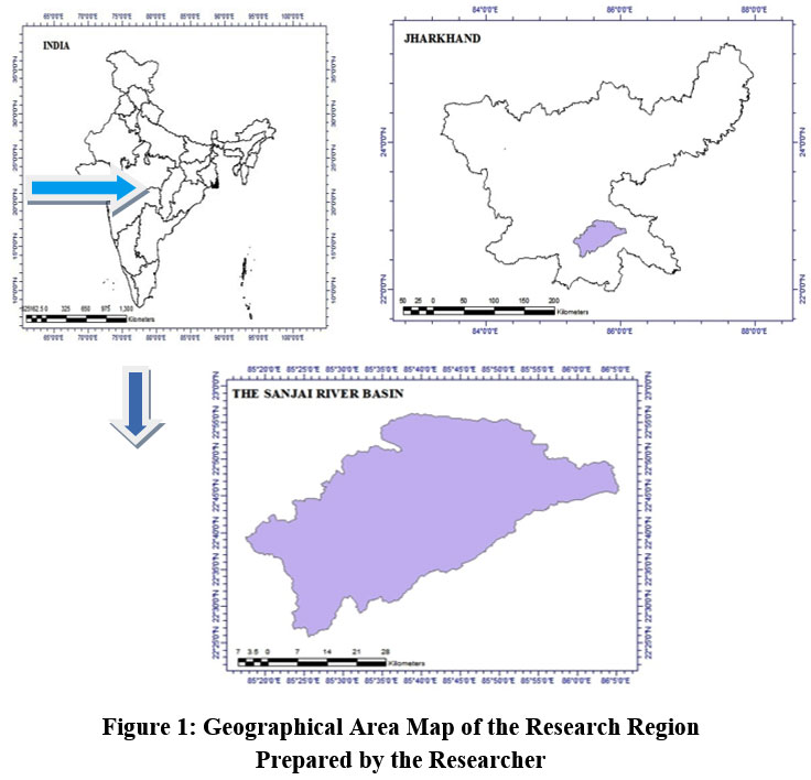Figure 1: Geographical Area Map of the Research Region. Click here to view Figure

Prepared by the Researcher

Methods and Materials

The SCS-CN runoff model technique consists of multiple segments. Listed below are the many methods that were provided earlier:

LULC map emerged from the Landsat 8 OLI satellite imagery, which was collected in April 2021. The NBSS and LUP furnished the soil surface map. IMD, Ranchi provided daily rainfall figures. A digital elevation model has been employed to create the watershed map.
Initially, Erdas Imagine 14 was employed to determine the LULC . The researcher subsequently transformed the published soil map into a computerized version of the soil surface map. Arc Gis 10.1 was used for generating the watershed map. Subsequently, the LULC map and the soil map were superimposed. After that, a number of micro watersheds were studied using the overlay LULC and soil map. In the region where I am investigating, there are nine micro watersheds. The Hydrological Soil Group (HSG) and a distinct LULC are used to figure out the curve number. Based on each CN and each LULC area, the weighted CN (WCN) is predicted.

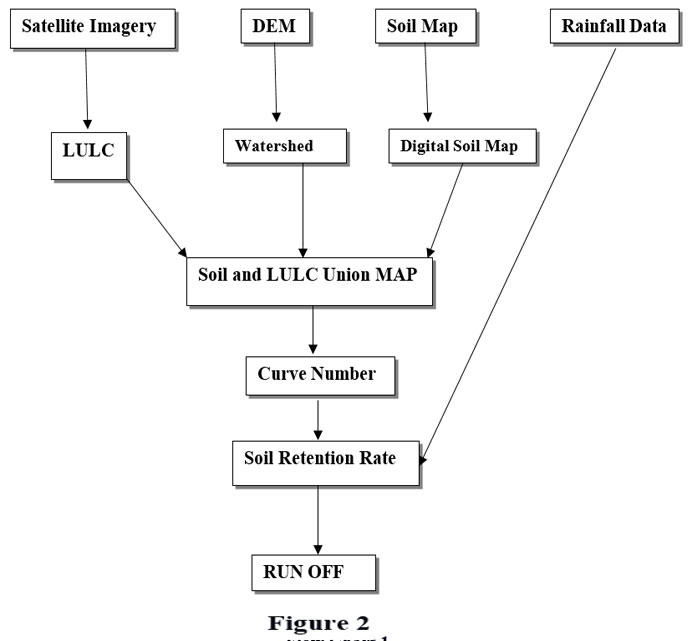Figure 2 Click here to view Figure

Weighted CN = (Area of Dense Vegetation X CN) + (Area of Crop Land X CN) + (Area of Settlement X CN)……………..(Area of Canal X CN) / (The overall surface of the Sub-Watershed)

The Soil Retention Rate has been determined by converting WCN with diversified Antecedent Moisture Conditions (AMC).

Finally, the Runoff volume of each sub-watershed has been determined by considering the Soil Retention Rate and antecedent rainfall volume

“SCS-CN Model”: Run-off computation in the world mostly uses SCS-CN models.

The formulae necessary to construct this model are as follows;

“F/S = Q /(P - Ia)” ………………………Equation 1.

The parameters described by F, S, Q, P, and Ia are the actual retention, prospective maximum retention, cumulative runoff, initial abstraction, accumulated downpour, appropriately, represented in millimeters.

Following the onset of precipitation, every further precipitation either becomes discharge or true retention.

“F = P – Ia – Q” ……………….Equation 2

After integrating all these equations

“Q equals (P-Ia)² / P-Ia + S”…… ………….Equation 3

In this context, Q symbolizes the sum of the runoff in millimeters, P defines the overall depth of downpour in millimeters, and Ia embodies the initial abstraction in millimeters, penetration, Surface storage and interception occur immediately before the commencement of the outflow in the catchment area. An equation has been devised to describe the initial abstractions. The relationship is,

Ia = 0.3(Considering the specific circumstances in India)

‘S’is the Possible highest retention rate and it is highlighted in the equation

“S = (25400/CN) – 254” ………………..Equation 4

CN is ranging from 0 to 100 where S = ? and S = 0 equivalently

“ (P-0.3S)² / (P-0.7S) = Q”.. ……………………..Equation 5

S stands for potential water retention, P as precipitation/ Downpour, and Q represents surface runoff volume in this particular instance.

This technique displays the suitability of soil for penetration of water related LULC and Conditions of Antecedent Moisture.
“As per US Soil Conservation Services, soil can be categorized into 4 hydrologic soil categories concerning the degree of potentiality and frequency of ultimate penetration.” (S. Satheeshkumar et al.2017)

“A trio of humid environments (AMC) occur on land,” according to CN. These are —

Arid State (CN I)( Wilting point not yet achieved)

Moderate State (CN II)

Condition of Saturation (CN III)

AMC I and III conditions are simply established via AMC II on the basis of curve numbers. “Using the following formulas helps one to ascertain the conditions for AMC-I and AMC-III.”(Chow et al.2002)

The formula for “CN(I) is 1/2 of CN(II) /2.281-0.0128CN(II)” ………….Equation 6

“CN(II)/0.427+0.00573CN(II)=CN(III)”……………….………Equation 7

Here, CN I, or the Arid State Curve Number

A moderate state's CN II is its curve number

CN III or the Saturation Condition Curve Number

Table 1: AMC Conditions

(Source: After Soil Conservation Service1972)

Hydrological Soil Group (HSG): SCS has devised a soil classification based on infiltration rate that consists of four distinct groups of soil. Such as :

‘A’ – Indicates the probability of minimal discharge and a high rate of penetration.

Shows a quite moderate rate of penetration and a rather fine to moderately deep texture in moderately drained to well-drained soil’.(USDA, NEH section 4, Hydrology).

It has an inefficient rate of infiltration when regularly wetted and a poor water transfer rate.

When completely wetted, it has the potential for substantial discharge and the infiltration rate is quite low.

Table 2: The group of Hydrological Soils

Source: Soil Conservation Service Classification, 1974

Now the Weighted curve number will be measured. The equation is presented below;

“Weighted Curve Number(WCN) = (CN*Area)/ Total Area ………….Equation 8

For the computation of the Depth of Surface Runoff, equations number 4 and 5 will be utilized.

Results And Discussion

Soil: Soil map has been collected from www.daas.ornl.gov.com and NBSSLUP. The hydrological soil group has defined four soil classes based on infiltration rate, Especially “A, B, C, and D”.

A soil group spreads across 823 sq km. of the research region. B soil group covers an area of 415 sq km., 289 sq km the region stands for soil group C and the expansion of D soil group is 743 sq km.

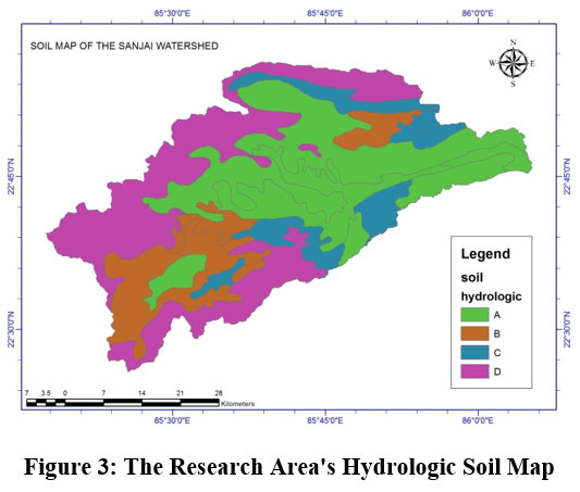Figure 3: The Research Area's Hydrologic Soil Map Click here to view Figure

Source : www.daac.ornl.gov.com and Eastern Region Office of NBSSLUP

LULC: The Supervised classification was used to create the LULC research map.. This technique resulted in the establishment of eleven classes. These are:
Dense vegetation occupies 668.97 sq.km. or 29.47% of the total area. 315.79 sq. km. or 13.97% of the total area, are presented with Fairly Dense Vegetation. 1137.95 sq.km., or 50.13% of the total area, are made up of cropland. Settlement 53.44 sq km (2.35% of total area). Lakes, ponds, reservoirs, and other bodies of inland water are examples of inland water bodies. It makes up 1.83% of the whole area, or 41.59 sq.km. With an area of 8.86 sq.km. the river makes up 0.39% of the whole. Comprising 0.05% of the total research area, the 1.12 square kilometer swamp has several hills and valleys that define the research area. This rocky outcrop encompasses around 32sq. km. area and 1.42% of the overall area. Fallow land is 0.68sq km. and 0.03% of the total area Build-up area is created by human activity. Nowadays this sort of area is expanding. In my study area, it comprises 9.07sq km. and 0.40% of the overall area. The canal is spreading across 0.35 sq km. area and 0.02% of the overall region.

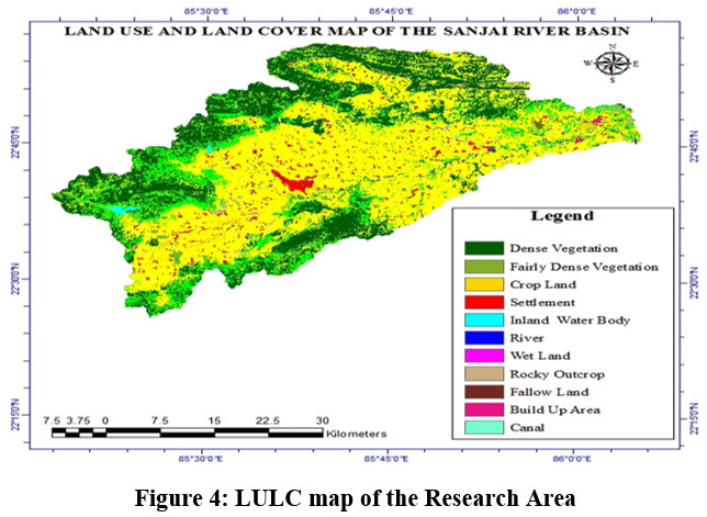Figure 4: LULC map of the Research Area Click here to view Figure

Source : Created by the Researcher

The Union tool in Arc Gis10.1 is used to merge the soil and LULC maps. Then, based on the various LULC and soil types, curve number values for Hydrologic soil cover complexes were allotted. The catchment region was now separated into 9 sub-watersheds, from which a combined soil and LULC map was produced.
The surface runoff volume is 981.85mm. Because the basin possesses secondary porosity, the runoff value is unusually high in contrast to annual rainfall, which is 1054.6mm. The following discussion indicates that the runoff characteristics are structurally regulated. The total quantity of runoff is bigger in hilly sub-watersheds as the slope amount is higher, infiltration becomes lower and lower in plain ones because of low degree of slope.

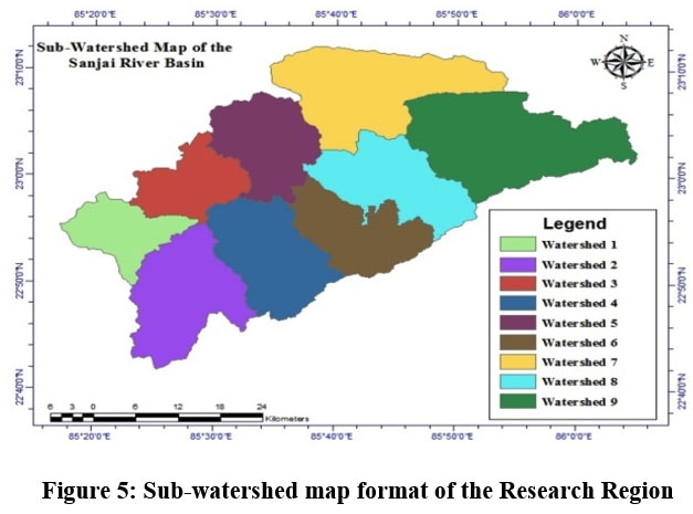Figure 5: Sub-watershed map format of the Research Region. Click here to view Figure

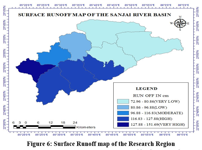Figure 6: Surface Runoff map of the Research Region Click here to view Figure

Source : Prepared by the Researcher

Table 3 : Run off Volume

Total Run off = 981.85mm.

Conclusion

The SCS-CN technique is effective for calculating surface runoff. This strategy may also be employed for watershed management. The quantity of runoff in the Sanjai River Basin fluctuates with deviations in LULC and soil conditions. According to the LULC map, agricultural land has the largest area of any class in the basin. According to the soil map, the soil category 'A' is the dominant soil in the basin. Finally, the SCS-CN Technique may be employed to locate artificial recharge locations that will be used as an irrigation source in agriculture.

Acknowledgement

The authors would like to thank teaching and non-teaching staff of the Department of Geography, Panskura Banamali College, Panskura for their kind contribution.

Funding Sources

The authors received no financial support for the research, authorship, and/or publication of this article.

Conflict of Interest

The authors declare no conflict of interest.

Author’s Contribution

Dr. Swati Mondal’s Contribution : My Supervisor has made the blueprint regarding the current research work and has guided me for the same and refined final manuscript.

Arunashis Chandra’s Contribution : I have worked on the framework decided by my supervisor and has made the graphs, maps and have interpreted and analyzed the results.

Data Availability Statement

The manuscript incorporates all dataset produced or examined throughout their research study.

Ethics Approval Statement

Not Applicable

References

1. Sarangi A, Bhattacharya AK. Comparison of artificial neural network and regression models for sediment loss prediction from Banha watershed in India. Agricultural Water Management.2005;78,pp195–208. DOI:10.1016/j.agwat.2005.02.001
   CrossRef
2. Hawkins RH. Improved prediction of storm runoff in mountain watersheds. J. Irrig. Drain. 1973.99(4) pp. 519-523. DOI:10.1061/JRCEA4.0000957
   CrossRef
3. Hawkins, R.H., 1993. Asymptotic determination of runoff curve numbers from data. J. Irrig. Drain. Eng. 119, 334-345. https://doi.org/10.1061/(ASCE)0733-9437(1993)119:2(334
   CrossRef
4. Hawkins RH, Ward TJ, Woodward DE, Van Mullem, JA.Curve cumber hydrology-State of practice. The ASCE/EWRI Curve Number Hydrology Task Committee.(2009) DOI:10.1061/9780784410042
   CrossRef
5. Sarangi A; Madramootoo C A; Enright P; Prasher S O; Patel R M.Performance evaluation of ANN and geomorphologybased models for runoff and sediment yield prediction for a Canadian watershed. Current Science.(2005)89(12), 2022–2033
6. Mohamad ES, Belal A, Mohamad A.Quantitative assessment of Surface runoff at arid region: a case study in the middle of Nile Delta.Bulletin of the National Research Centre. (2019).43:186 . https://doi.org/10.1186/s42269-019-0230-7
   CrossRef
7. Patel J, Singh NP, Prakash I, Mehmood K .Surface Runoff Estimation Using SCS-CN method- A Case study on Bhadar Watershed, Gujrat, India.Imperial Journal of Interdisciplinary Research.(2017). 3(5):1213-1218
   CrossRef
8. Patil J.P., Sarangi A., Singh A.K., Ahmed T.(2008).Evaluation of modified CN methods for watershed runoff estimation using a GIS-based interface. Biosystems Engineering.100:137-146
   CrossRef
9. Shadeed Sameer, Almasri Mohammad(2010). Application of GIS-based SCS-CN method in West Bank catchments, Palestine. Water Science and Engineering.3(1):1-13
10. United States Department of Agriculture (USDA). National Engineering Handbook. Section 4. Hydrology. Washington, DC: Soil Conservation Service, US Government Printing Office; 1972.
11. United States of Department of Agriculture (USDA), National Engineering Handbook of Hydrology, 1972. Handbook Section-4, Chapter-21.
12. United States of Department of Agriculture (USDA). National Engineering Handbook of Hydrology Part 630. Natural Resources Conservation Service. Chapter10.2004
13. Hydrology Task Committee. Hawkins, RH, Ward, TJ, Woodward, DE, Van Mullem, JA, 2010. Continuing evolution of rainfall-runoff and the curve number precedent. In: 2nd Joint Federal Interagency Conference, Las Vegas, NV
14. Satheeshkumar S., Venkateswaran S., Kannan R. Rainfall-Runoff estimation using SCS-CN and GIS approach in the Pappiredipatti watershed of the Vaniyar sub basin, South India. Model. Earth Syst. Environ. (2017) .3:24. DOI 10.1007/s40808-017-0301-4
    CrossRef
15. Chow, V.T., Maidment, D.R., Mays, L.W., 1988. Applied Hydrology. McGraw-Hill, New York.